Excel Challenge 32 : Identify Top 3 Sales Performers

The Problem

Top-performer lists are easy to describe and easy to get wrong by hand. Once several agents are involved, scanning the numbers and deciding who belongs in the top three becomes a lot less reliable than it sounds.

The risk is not just picking the wrong winner. A report also needs a repeatable cutoff so the top group can be marked again when revenue changes. The worksheet should decide the top three from the data, not from a one-time manual sort.

The flow below shows how the cutoff drives the whole report. Once the third-highest revenue is known, each row can be tested against it and the summary can count and total the winning group.

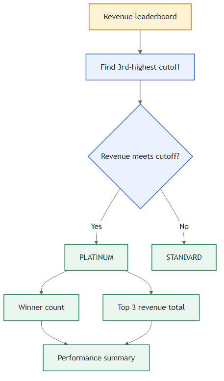The Problem: Top Performer Lists Need a Repeatable Cutoff The third-highest value becomes the entry bar for the winner group.

In this workbook, each sales agent has one revenue value. The challenge is to flag the top three earners, total the revenue from that group, and count how many winners were found in the table.

The cutoff should come from the revenue list itself.
The row labels should identify the top performer group.
The summary should total and count only the winner rows.

That keeps the leaderboard easy to update. If the numbers change later, the cutoff, labels, and summary can all recalculate together.

How We Solve It

The cleanest shortcut is to find the third-largest revenue and use it as the entry bar. Anyone whose revenue is greater than or equal to that value belongs in the top group. After that, the summary cells become straightforward.

Method 1: Use LARGE as the cutoff

Method 1: Use the third-highest value as the cutoff for the top group.

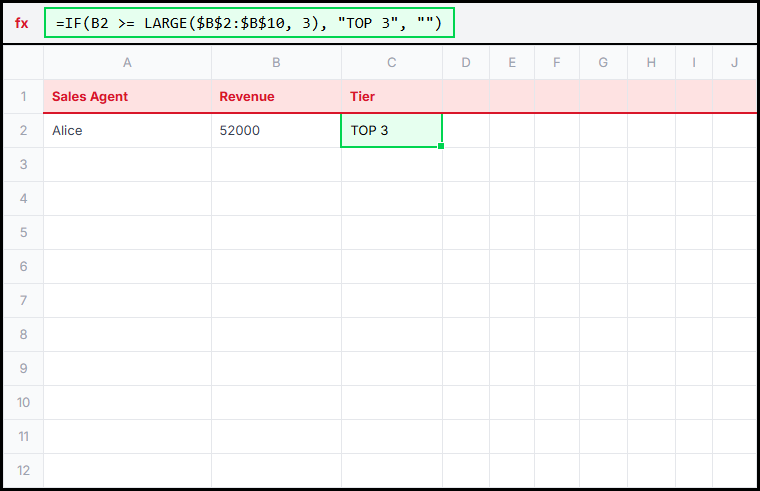
This is the method used in the solution. LARGE($B$2:$B$6, 3) returns the third-highest revenue. Once we have that benchmark, IF can mark each row as PLATINUM or STANDARD.

This solves the challenge because the worksheet needs one clear cutoff that defines who belongs in the top three. Once the third-highest revenue is known, every row can be tested against that single benchmark without sorting the table by hand.

=IF(B2 >= LARGE($B$2:$B$6, 3), "PLATINUM", "STANDARD")

Method 2: Rank every agent

Method 2: Assign each agent a position in the leaderboard.

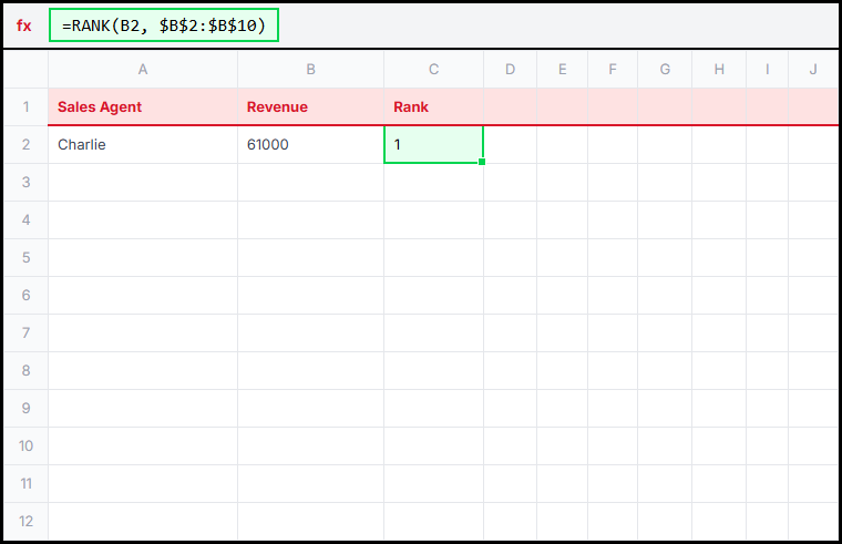
RANK is useful when you want to see each agent's exact position instead of just whether they made the cut. It is not the formula pattern used by the validator, but it is a natural companion to the same top-three logic.

This solves a more detailed version of the leaderboard problem. Instead of only telling us whether someone made the top group, it shows each agent's standing, which is useful when the report needs full ranking information.

=RANK(B2, $B$2:$B$6)

Method 3: Build a separate winners list

Method 3: Create a separate winners list with sorting functions.

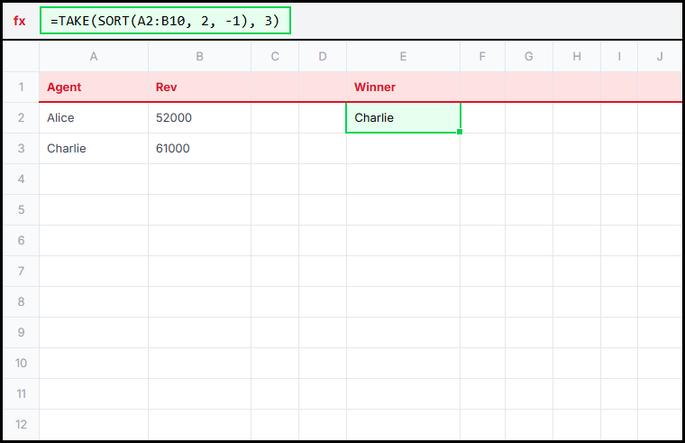
Modern Excel can also sort the table and return only the top rows. That is helpful when a report needs a separate winners section instead of labels inside the main table.

This solves the reporting problem when the business wants a standalone winners list. After sorting the table by revenue, the formula can return only the top performers without changing the original data block.

=TAKE(SORT(A2:B6, 2, -1), 3)

Function Explanation

1. LARGE

LARGE returns the nth largest value in a range. In this challenge it provides the exact revenue threshold that defines who belongs in the top three.

That threshold is what makes the report repeatable. The sheet can identify the winner group without sorting the original data block.

Learn more this functionLARGE

2. IF

IF turns the threshold comparison into a visible category label. That is what makes the ranking easy to read in the main table.

Once the row says PLATINUM or STANDARD, the summary can use those labels without repeating the ranking logic.

Learn more this functionIF

3. SUMIFS

SUMIFS adds only the revenue rows that match the PLATINUM label. That gives the summary total for the winners without extra helper columns.

This keeps the summary tied to the visible classification column, which makes the report easier to audit.

Learn more this functionSUMIFS

Ties are the one thing to think about in real leaderboards. If several people share the third-highest value, a cutoff formula can include more than three winners, which may or may not be what the business wants.