Excel Challenge 33 : Remove Non-Numeric Characters

What You Will Learn

Five raw invoice amounts in A2:A6: "$1200.00", "500 USD", "Price: 15.50", "2500.00 each", "TOTAL 45.00". Each has extra text around the number. You need to strip everything except the numeric value and convert the result to a real number in column B.

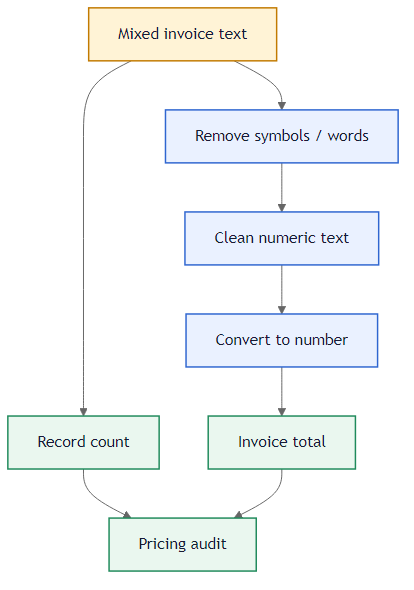
Use SUBSTITUTE to remove known text pieces, then VALUE to convert the cleaned text to a number:

=VALUE(SUBSTITUTE(SUBSTITUTE(SUBSTITUTE(SUBSTITUTE(A2,"$",""),",",""),"USD",""),"Price:",""))

Each SUBSTITUTE targets one unwanted piece. "$1200.00" → remove $ and commas → "1200.00". "500 USD" → remove "USD" → "500". "Price: 15.50" → remove "Price:" → " 15.50" → VALUE converts to 15.5. The same chain handles "2500.00 each" and "TOTAL 45.00" by also stripping "each" and "TOTAL". The VALUE wrapper ensures the result is a real number, not text that looks numeric.

Without VALUE, the cleaned result might look like a number but still be stored as text. SUM ignores text values, so the audit total would be wrong. VALUE forces Excel to treat the cleaned string as an actual number that can be calculated.

SUBSTITUTE removes unwanted text. VALUE converts to a real number.

The audit formulas:

B9: =COUNTA(A2:A6) — total records processed.
B10: =SUM(B2:B6) — total invoice sum after cleanup.

Alternative: NUMBERVALUE for Currency Formats

If data uses consistent separators: =NUMBERVALUE(A2,".",","). Handles the dollar sign row in one step but not word labels like "USD".

Going Further: Clean Once, Calculate Often

Once cleaned, store numeric values in a dedicated column. Raw data stays in column A for reference; clean numbers in column B drive every calculation.

The order of SUBSTITUTE calls does not matter as long as each call removes a specific piece of text. However, chaining too many SUBSTITUTE calls makes the formula hard to read. For files with many inconsistent patterns, it is often faster to use Find & Replace or Power Query to standardize the data before applying a simpler formula.

The chained SUBSTITUTE approach removes only what you specify. If a new row contains unexpected text (e.g., "EUR 500"), add another SUBSTITUTE to the chain. For complex cleanup, Power Query may be better.