What You Will Learn
You have two lists. The official holiday registry is in F2:F4 (Jan 1, July 4, Dec 25). Your service dates are in A2:A6. You need to label each service date as "HOLIDAY" or "WORK DAY" in column C.
This is an existence check — does a value from one list appear in another? COUNTIF is the simplest tool for this:
=IF(COUNTIF($F$2:$F$4, A2) > 0, "HOLIDAY", "WORK DAY")
COUNTIF counts how many times the date in A2 appears in the holiday range. If the count is greater than 0, the date is a holiday. The $F$2:$F$4 has dollar signs so the range stays locked when you fill the formula down.
In this dataset: Jan 1 (New Year Day) and Dec 25 (Christmas Day) are holidays. July 4 (Independence Day) is also a holiday. Jan 5 and Mar 15 are not in the registry, so they are work days. That gives 2 holidays out of 5 service dates.
The dollar signs around the registry range ($F$2:$F$4) are essential here. Without them, filling the formula down would shift the range — C3 would check F3:F5 instead of F2:F4, missing the holiday at the top of the list and potentially picking up an empty cell at the bottom.
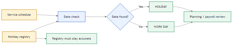 COUNTIF checks each service date against the holiday registry.
The audit formulas:
- B9:
=COUNTA(A2:A6) — total service dates reviewed.
- B10:
=COUNTIF(C2:C6,"HOLIDAY") — how many holidays were found.
Alternative: MATCH + ISNUMBER
Instead of COUNTIF, you can use MATCH to search the registry:
=IF(ISNUMBER(MATCH(A2,$F$2:$F$4,0)),"HOLIDAY","WORK DAY")
MATCH returns a number if it finds the date, or an error if it does not. ISNUMBER converts that into TRUE/FALSE. Same result, different approach.
Going Further: Holiday Names
If you need the holiday name instead of just a flag, expand the registry to include names (G2:G4) and use VLOOKUP:
=VLOOKUP(A2,$F$2:$G$4,2,FALSE)
This returns "New Year Day", "Independence Day", etc. instead of a generic HOLIDAY label.
The 0 in MATCH (or the >0 in COUNTIF) forces exact matching. Without it, a close date could incorrectly match. For dates and IDs, always use exact match.
Check each service date against the holiday registry in F2:F4, mark the row as HOLIDAY or WORK DAY, and then finish the summary so the sheet shows how many records were reviewed and how many holidays were found.