What You Will Learn
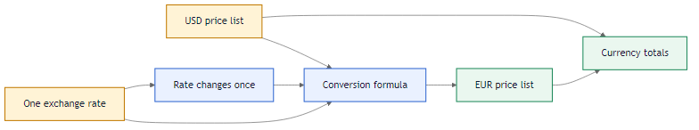
Five products with USD prices in B2:B6. The exchange rate (0.92 USD→EUR) is in G1. You need EUR prices in column C and totals for both currencies.
The formula is simple multiplication. The important part is locking the rate cell so every row uses the same value:
=B2 * $G$1
The dollar signs on $G$1 make it an absolute reference. Without them, copying the formula down would shift the reference: C3 would look at G2 (empty), C4 at G3 (also empty), and so on. With $G$1, every row points to the same rate.
 One rate cell drives every row. Update G1, and the whole column recalculates.
The audit formulas:
- B9:
=SUM(B2:B6) — total USD value before conversion.
- B10:
=SUM(C2:C6) — total EUR value after conversion.
The two totals side by side let you verify the conversion at a glance. If the rate changes, both sums update automatically because both columns depend on the same $G$1 cell.
What If You Need to Convert Back?
If you have EUR amounts and need to recover the original USD, reverse the math:
=C2 * (1 / $G$1)
Or divide instead of multiplying: =C2 / $G$1. Both return the same result. This is useful in audit work when you inherit the converted column first and need to verify the original amounts.
What Happens Without the Dollar Signs
If you write =B2*G1 (no absolute reference) and fill down:
- Row 2: B2*G1 ✓
- Row 3: B3*G2 → G2 is empty, result is 0
- Row 4: B4*G3 → G3 is empty, result is 0
Every row after the first would show zero — a silent error that looks like valid data.
In this dataset, the first product (Pro Laptop at $1,200) converts to €1,104 (1200 × 0.92). The last product (Server Unit at $3,000) converts to €2,760. If you forget the dollar signs, the formula would return €1,104 for the first row, then €0 for every row after — because each row would reference an empty cell instead of G1.
Absolute references are the difference between a sheet that works once and a sheet that keeps working. If the exchange rate changes next quarter, you edit G1 — not every formula in column C.
Use =B2*$G$1 in C2:C6 to convert USD to EUR. Then SUM in B9 for USD total and B10 for EUR total. Remember the dollar signs!