What You Will Learn
Five products have net prices in B2:B6. The tax rate (8.25%) is stored in G1. You need the tax amount per product in column C, the gross total in column D (net + tax), and the overall net and gross sums.
The main challenge is not the math — it is making sure every row uses the same tax rate even when the formula is copied down. That is what absolute references solve.
Step 1 — Tax amount (C2:C6):
=B2*$G$1
The dollar signs on $G$1 lock the reference. Without them, copying the formula down would shift the rate reference: C3 would look at G2 (empty), C4 at G3 (also empty), and so on. With $G$1, every row points to the same cell.
Step 2 — Gross total (D2:D6):
=B2+C2
Net price plus tax amount. Simple addition. The tax is kept visible in its own column so the reviewer can see exactly how much tax was added to each product.
Step 3 — Summary (B9, B10):
- B9:
=SUM(B2:B6) — total net value before tax.
- B10:
=SUM(D2:D6) — total gross value after tax.
The difference between these two numbers is the total tax collected across all products.
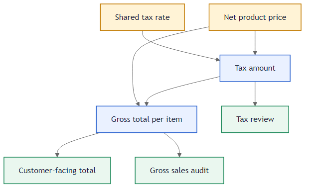 Net price × absolute rate reference → tax amount → gross total. One rate cell drives all rows.
What Happens Without Absolute References
If you wrote =B2*G1 (no dollar signs) and filled it down, here is what would happen:
- B2*G1 → correct
- B3*G2 → G2 is empty, result is 0
- B4*G3 → G3 is empty, result is 0
This is the most common mistake in this challenge. The dollar signs are the difference between a working sheet and one with silent errors.
Shortcut: One-Step Gross Total
If you only need the final amount, multiply the price by 1 + rate:
=B2*(1+$G$1)
This calculates the gross total directly without a separate tax column. It is useful for quick quotes, but the separate-column approach is better when you need to show the tax amount explicitly.
The most common error in this challenge is forgetting the dollar signs. Double-check that $G$1 stays the same in every row. If the results look wrong, that is the first place to look.
Use B2*$G$1 in C2:C6 to calculate tax per product, then =B2+C2 in D2:D6 for gross totals. Finish with SUM in B9 (net) and B10 (gross). Remember the dollar signs!