Excel Challenge 34 : Find the Second Best Sale

What You Will Learn

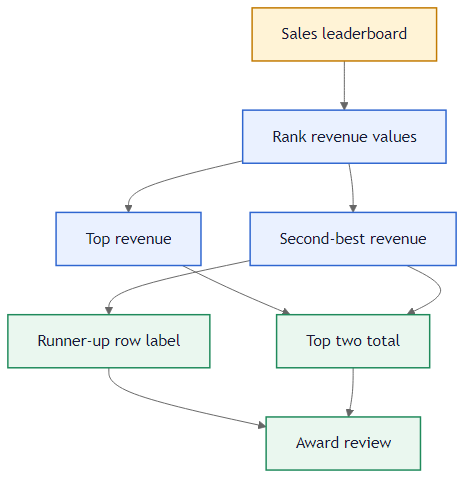
Five sales agents with revenue values. You need to find the second-best (runner-up) amount, flag the correct agent row, and total the top two revenues.

B10 — Runner-up revenue:

=LARGE($B$2:$B$6, 2)

LARGE returns the nth largest value. With position 2, it returns 59,000 (Diana's revenue). The dollar signs lock the range so the formula works correctly. If you changed the position to 1, you would get the top revenue (61,000). Position 3 would give the third-best (52,000). LARGE makes any rank accessible without sorting.

C2:C6 — Runner-up row label:

=IF(COUNTIF($B$2:$B$6,">"&B2)+1=2,"RUNNER UP","STANDARD")

COUNTIF counts how many revenues are higher than the current row. Adding 1 gives the row's rank. If the rank equals 2, the agent is the runner-up. Charlie (61,000) is first — nothing is higher, COUNTIF returns 0, +1 = 1. Diana (59,000) has exactly one higher value, COUNTIF returns 1, +1 = 2 — RUNNER UP.

B9 — Top two total: =LARGE(B2:B6,1)+LARGE(B2:B6,2) = 61,000 + 59,000 = 120,000.

LARGE finds the runner-up value. COUNTIF with rank logic flags the right row.

The B9 formula adds LARGE(B2:B6,1) and LARGE(B2:B6,2) — two separate calls to LARGE that return first and second place independently. This is more readable than a single complex formula because each part has a clear purpose: position 1 plus position 2.

Alternative: SORT + INDEX for the Name

If you also need the runner-up name: =INDEX(SORT(A2:B6,2,-1),2,1). Sorts by revenue descending, returns the name from the second row.

The COUNTIF formula uses ">"&B2 to count higher values. The ampersand joins the > operator with the cell reference. This dynamic comparison works on every row because B2 changes as the formula is filled down — each row counts how many values are higher than its own revenue, without needing a separate threshold cell.

If two agents have the same revenue, LARGE(...,2) still returns that value but COUNTIF with > may rank them both as position 2. In real leaderboards, decide how ties should be handled before building the ranking logic.

The COUNTIF formula uses ">"&B2 syntax to compare dynamically. The ampersand joins the comparison operator with the cell reference, so each row counts higher values relative to its own revenue without a separate helper cell.