Excel Challenge 32 : Calculate Discount Based on Category

What You Will Learn

Five products. Each has a category (Electronics, Furniture, or Clothing) and a base price. You need to calculate the discount amount in column D using the right rate for each category:

Category	Discount Rate
Electronics	5%
Furniture	20%
Clothing	15%

IFS checks the category and applies the matching rate in one formula:

=IFS(B2="Electronics",C2*0.05,B2="Furniture",C2*0.2,B2="Clothing",C2*0.15)

IFS reads each condition left to right. For a Furniture item, the first condition (Electronics) is false, the second (Furniture) is true, so it returns C2*0.2. Text labels must match exactly — "Furniture" in the formula must match "Furniture" in the cell.

Monitor 4K (Electronics, $300) gets $15 discount. Oak Desk (Furniture, $450) gets $90. Winter Coat (Clothing, $120) gets $18. Smartphone ($800) gets $40. Coffee Table ($150) gets $30. Total discounts: $193.

The formula needs the category text to match exactly. If the cell says "Electronics" but the formula checks for "electronics" (lowercase), it would not match and IFS would return an error. The same applies to extra spaces — "Furniture " with a trailing space would fail to match "Furniture".

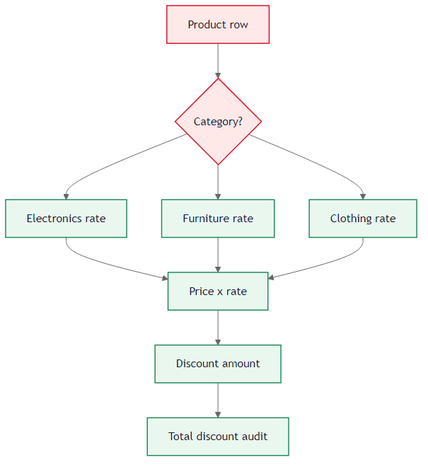IFS matches the category, applies the rate, and calculates the discount.

The audit formulas:

B9: =COUNTA(A2:A6) — total products.
B10: =SUM(D2:D6) — total discount value across all products.

Alternative: SWITCH

SWITCH separates the category matching from the calculation:

=C2*SWITCH(B2,"Electronics",0.05,"Furniture",0.2,"Clothing",0.15)

SWITCH returns the rate, then the multiplication happens once. Cleaner when multiple formulas use the same rate lookup.

Going Further: Rate Lookup Table

If rates change often, store them in a separate table and use VLOOKUP:

=C2*VLOOKUP(B2,$F$2:$G$4,2,FALSE)

Update the table instead of editing formulas. Best for workbooks where non-technical staff maintain the rates.

The IFS formula checks conditions left to right and stops at the first match. That means if you accidentally typed "Electronic" instead of "Electronics", the formula would skip that condition and potentially fall through to an incorrect match or return an error. Double-check category spelling against the actual data values.

The most common mistake is writing the rate as a whole number (15) instead of a decimal (0.15). A rate of 15 would multiply the price by 1500%, not 15%. Always test with a simple price like $100 — the result should be $15 for 15%, not $1,500.