What You Will Learn
You have five students. Each has a midterm score and a final score. The pass mark is 70. You need to calculate each student's average, label them PASS or FAIL, and count how many passed.
The decision chain works like this: scores → average → compare against 70 → show PASS or FAIL → count the results. That is two row-level formulas (AVERAGE and IF) followed by two summary formulas.
The data:
B2:C6 — midterm and final scoresD2:D6 — your AVERAGE formula goes hereE2:E6 — your IF formula goes hereB9 — total student countB10 — passing count
The Formulas
Step 1: Average the Scores
Each student has two scores. AVERAGE adds them and divides by two in one step:
=AVERAGE(B2:C2)
Fill this down from D2 to D6. The result is the combined performance for each student — 88.5 for Alice, 65 for Bob, and so on.
Step 2: Apply the Pass Mark
IF checks whether the average meets 70. If it does, the cell shows PASS. If not, it shows FAIL:
=IF(D2>=70,"PASS","FAIL")
Fill this down from E2 to E6. The pass mark (70) lives in cell H1 — if the threshold ever changes, you update H1 instead of editing every formula.
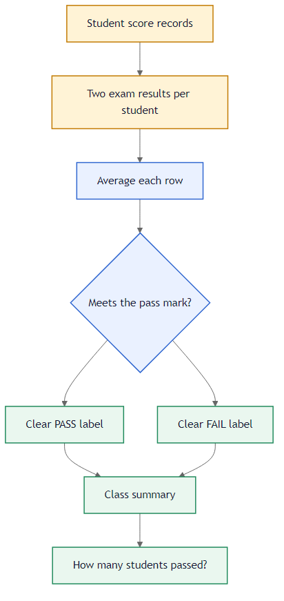 Scores become averages, averages become pass/fail labels, labels become summary counts.
Step 3: The Summary
- B9:
=COUNTA(A2:A6) — counts how many students are in the roster.
- B10:
=COUNTIF(E2:E6,"PASS") — counts how many earned PASS.
COUNTA is used here instead of COUNT because student names are text, not numbers. COUNT only counts numeric cells; COUNTA counts any non-empty cell. COUNTIF then narrows the total down to just the passing students.
Going Further: One-Formula Shortcut
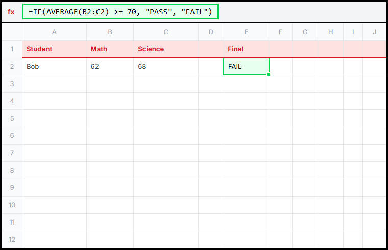
If you only need the final label and not the intermediate average, you can nest AVERAGE inside IF:
=IF(AVERAGE(B2:C2)>=70,"PASS","FAIL")
This saves a column but hides the average from view. The two-column approach is better when someone needs to verify the score behind the decision.
 Nesting AVERAGE inside IF saves space but hides the intermediate number.
Going Further: Letter Grades with IFS
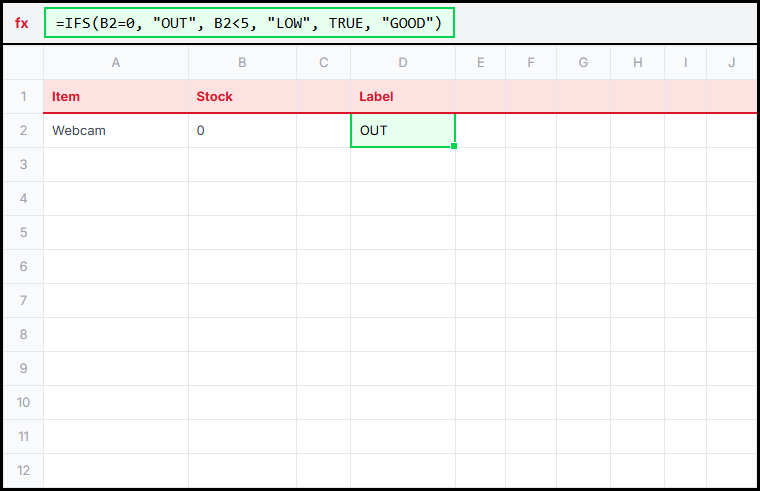
If the sheet later needs A/B/C/D/F grades instead of pass/fail, IFS replaces IF and checks multiple bands in order:
=IFS(D2>=90,"A",D2>=80,"B",D2>=70,"C",TRUE,"F")
The higher bands must come first — otherwise a student with 92 could match the "B" threshold before Excel reaches "A".
 IFS handles multiple grade bands in a single formula.
The pass mark is stored in H1 instead of being typed into the formula. That means if the threshold changes next semester, you edit one cell instead of every row.
Use AVERAGE in D2:D6 to calculate each student's combined score, then IF in E2:E6 to label PASS or FAIL. Finish with COUNTA in B9 for total students and COUNTIF in B10 for passing count.