Excel Challenge 39 : Flag High-Value Customers

What You Will Learn

Six orders. Some customers appear multiple times — John Doe ordered twice ($2,500 + $3,000). A single order might be small, but the combined total could still be high. You need to label each row as VIP if the customer's total spending exceeds $5,000.

SUMIF adds all orders for the same customer, then IF checks the total against the threshold:

=IF(SUMIF($A$2:$A$6, A2, $B$2:$B$6) > 5000, "VIP", "STANDARD")

SUMIF looks at every occurrence of the name in A2 across the entire column A, then adds the corresponding amounts from column B. For John Doe on row 2, it finds rows 2 and 4 — $2,500 + $3,000 = $5,500. That exceeds $5,000, so the label is VIP.

The dollar signs ($A$2:$A$6) lock the lookup range. Without them, filling the formula down would shift the range — C3 would check A3:A7 instead of A2:A6, missing John's first order on row 2 and potentially reading empty cells at the bottom. The absolute reference is essential for SUMIF to work correctly across all rows.

John Doe ($5,500) and Jane Smith ($6,000) are VIPs. Bob Brown ($1,200) and Alice Green ($4,800) are STANDARD. Note that all of John's rows show VIP and all of Bob's rows show STANDARD — the label is consistent per customer because SUMIF looks at the full customer total.

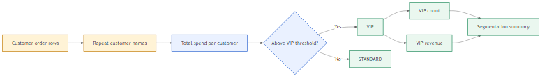SUMIF aggregates all orders per customer. IF checks against the VIP threshold.

The audit formulas:

B9: =COUNTIF(C2:C6,"VIP") — count of VIP rows.
B10: =SUMIF(C2:C6,"VIP",B2:B6) — total revenue from VIP rows.

Going Further: Multiple Tiers

If you need Silver, Gold, Platinum tiers instead of VIP/STANDARD, combine SUMIF with a lookup table: =VLOOKUP(SUMIF($A$2:$A$6,A2,$B$2:$B$6),$E$2:$F$5,2,TRUE). Store the tier thresholds in a small table. Update the table when thresholds change — no formula editing needed.

The COUNTIF in B9 counts VIP rows, not unique VIP customers. If John Doe appears twice and both rows are VIP, the count is 2 — not 1. If you needed unique customer count instead of row count, you would use a different approach like counting distinct names where the category is VIP.

The $5,000 threshold is a business rule, not a formula requirement. Change it to $3,000 or $10,000 and the labels update automatically — only the number in the IF statement changes.