OFFSET Dynamic Range Reference Formula
Learn how to construct dynamic ranges in Excel using OFFSET. Build rolling 3-month averages, flexible financial models, and understand volatility risks cleanly.

Financial analysts calculating rolling 3-month averages or inventory buffers face a constant challenge: each time a new month is appended to the bottom of the table, static formulas like =AVERAGE(B4:B6) must be updated by hand to cover the latest period.
The OFFSET formula acts as a flexible anchor. It starts at a base cell and shifts down and across by a designated number of rows and columns, dynamically resizing to create new ranges.
Syntax and the Five Arguments
=OFFSET(reference, rows, cols, [height], [width])- reference: The starting anchor cell (e.g.
A1orB1). - rows: Number of rows to move down (positive) or up (negative).
- cols: Number of columns to move right (positive) or left (negative).
- height: Optional number of rows high the returned range should be (default 1).
- width: Optional number of columns wide the returned range should be (default 1).
Constructing Dynamic Rolling Averages
By nesting OFFSET inside AVERAGE or SUM, you can instruct Excel to aggregate a floating window of cells:
=AVERAGE(OFFSET(B1, 3, 0, 3, 1)) // Averages 3 rows starting from row 4Volatility Warning
Just like INDIRECT, OFFSET is a volatile formula that recalculates whenever any cell in the workbook changes. Use it for dashboard KPI summary cards, but avoid applying it across hundreds of thousands of ledger entries.
Hands-on Practice Playground
Use the monthly revenue ledger below to test dynamic coordinate shifting and rolling averages using OFFSET. Follow each objective to complete the exercise.
In cell E2, retrieve the sales revenue for March starting from anchor A1 and shifting by row D2 and column D3.
In cell E2, retrieve the sales revenue for March by starting at anchor cell A1 and shifting downwards by row offset D2 and rightwards by column offset D3 using OFFSET.
In cell F2, calculate the 3-month moving average of March through May using AVERAGE and OFFSET.
In cell F2, calculate the 3-month moving average of the latest three months (March to May) by wrapping an AVERAGE formula around OFFSET anchored at B1, shifted down 3 rows, with a height of 3 rows and width of 1.
In cell F3, calculate the average for January through March.
In cell F3, calculate the average for January through March by wrapping AVERAGE around OFFSET starting at B1, shifted down 1 row, with height 3 and width 1.
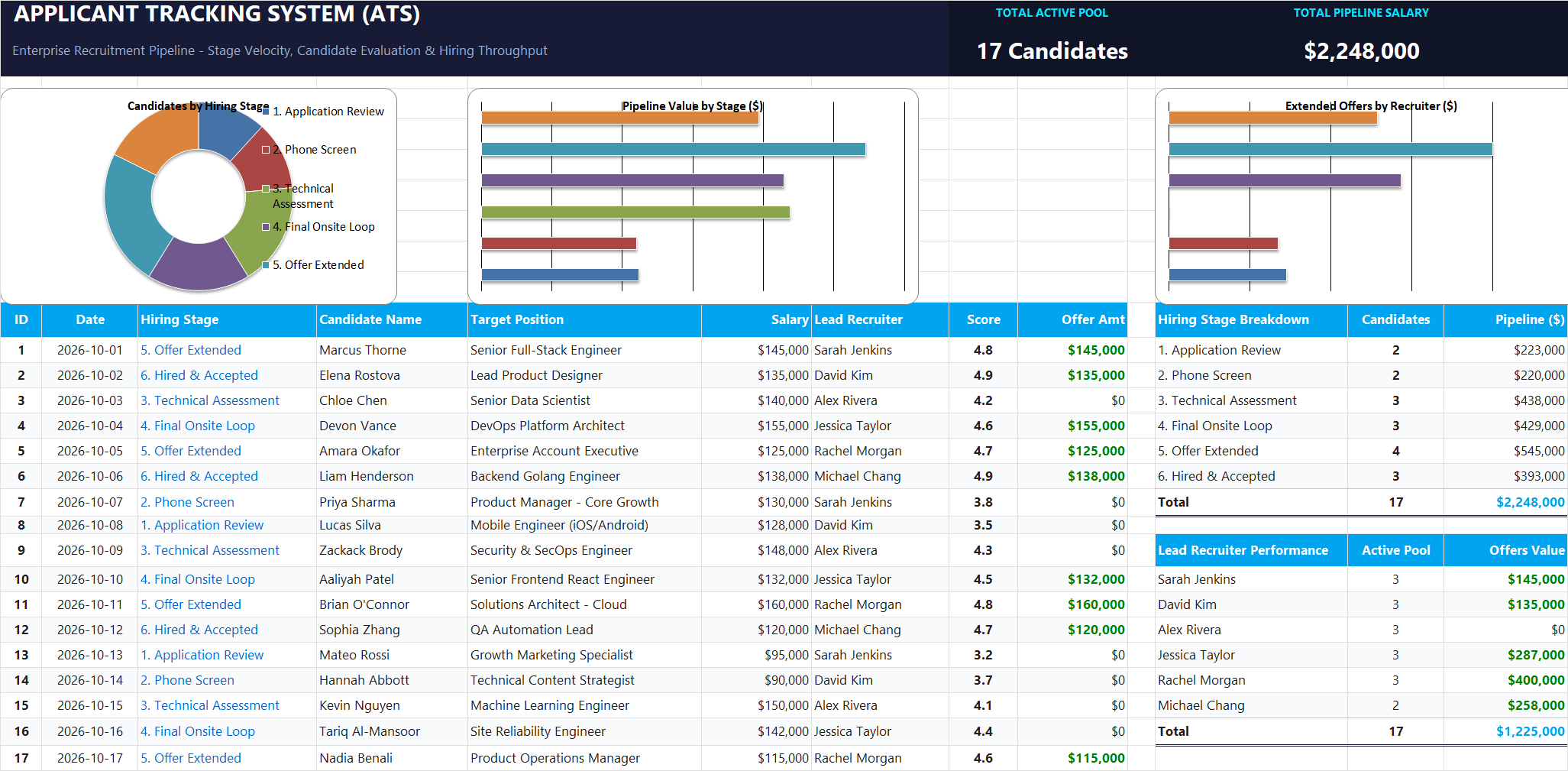
Ready to apply OFFSET Dynamic Range Reference Formula in a real workbook?
Apply lookup and reference formulas to search and organize structured candidate pipelines.
Open Applicant Tracking System (ATS)Share This Lesson
Spread the word with your peers and challenge your friends