If you have ever coordinated hiring for a growing team, you know how quickly spreadsheet chaos happens. One recruiter types "Interview", another writes "Stage 2 Phone Screen", and candidate scores sit scattered across random notes. Before you know it, leadership asks for an update on open offers, and you spend half your Friday manually fixing broken formulas.
In this practical tutorial, we will build a clean, reliable Applicant Tracking System (ATS) in Microsoft Excel from start to finish. You will see how simple dropdowns keep your team from making typos, how a basic IF rule approves job offers automatically, and how COUNTIF and SUMIF tally candidate counts and total salary commitments in real time.
Laying Out the Candidate Tracker
Before writing formulas, let us organize our sheet so it stays clean even when you are juggling dozens of open roles. We divide our single worksheet into three clear areas: the summary banner up top (rows 2 to 4), the main candidate list in the middle (columns D to L, rows 13 to 30), and our summary tables on the right (columns N to P).
This layout keeps things simple: your recruiters can log applicants row by row during daily standups, while department leaders can glance at the top banner and immediately see total active applicants and budget commitments.
Here is how columns D through L organize candidate details across rows 14 to 30:
| Col | Field Name | Type | Format | Operational Role |
|---|---|---|---|---|
| D | ID | Integer | 1, 2, 3... | Unique applicant number for each candidate in the pipeline. |
| E | Date | Date | YYYY-MM-DD | The date the application was received. |
| F | Hiring Stage | Dropdown | List Data Validation | Current recruitment step (from 1. Application Review to 6. Hired & Accepted). |
| G | Candidate Name | Text | Title Case | Full candidate name (for example, Marcus Thorne or Elena Rostova). |
| H | Target Position | Text | Job Title | Role title (such as Senior Full-Stack Engineer or Lead Product Designer). |
| I | Salary | Currency | $#,##0 | Annual salary requested by the candidate. |
| J | Lead Recruiter | Text | Staff Name | Team member responsible for guiding the candidate through interviews. |
| K | Score | Decimal | 0.0 | Interview scorecard rating on a friendly 1.0 to 5.0 scale. |
| L | Offer Amt | Formula | $#,##0 | Approved offer amount calculated with =IF(K14>=4.5, I14, 0). |
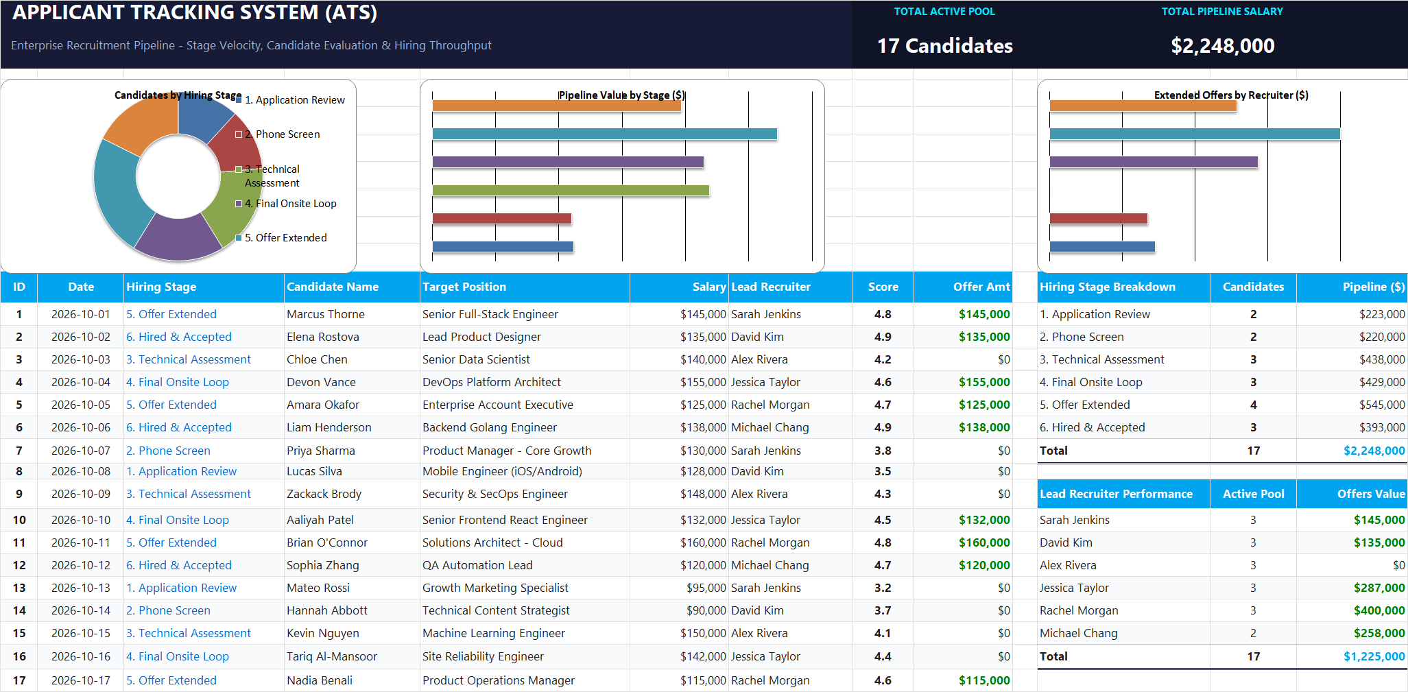
Figure 1: The unified ATS layout with our top dark navy summary banner, candidate list, and summary tables on the right.
Now that our candidate table is ready, let us set up our first safeguard to keep everyone entering stages the exact same way.
Setting Up Dropdowns and Automatic Offer Approvals
A good tracker should do the heavy lifting for you while preventing silly mistakes. In this section, we will lock the stage column to clean dropdown choices and let Excel decide when a candidate qualifies for an official offer.
Notice how Chloe Chen in row 16 earned a score of 4.2. Because 4.2 is below 4.5, cell L16 safely returns $0, preventing unauthorized verbal offers from slipping through.
1Action: Adding Stage Dropdowns with Data Validation
When several people edit the same spreadsheet, small typos are inevitable. If someone writes "Offer" while someone else writes "5. Offer Extended", formulas like COUNTIF treat them as completely different stages and your totals get thrown off.
To fix this permanently, we lock cells F14:F30 with an in-cell dropdown list. Select cells F14:F30, go to the Data tab on the Ribbon, click Data Validation, choose List under Allow, and paste our six standard stage names into the Source box.
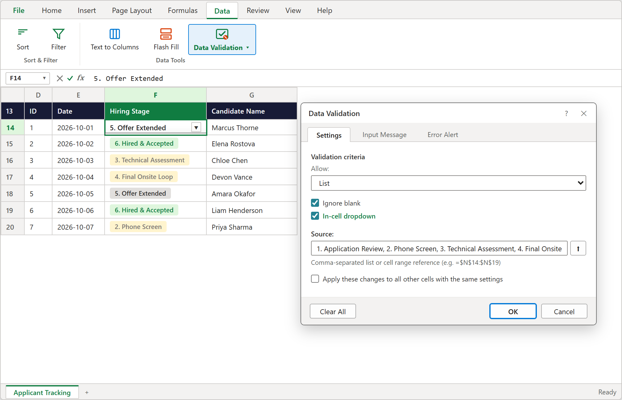
Figure 2: Setting up Data Validation so recruiters can pick stages directly from a clean in-cell dropdown.
2Action: Auto-Approving Offers with the IF Formula
Before your team extends an official job offer, you want to make sure the candidate passed their interview loop with flying colors. In our team rubric, applicants need a score of 4.5 or higher out of 5.0 to receive an approved salary offer.
Instead of checking every score by hand, let Excel do the math. In cell L14, enter this simple condition:
3Result: Making Numbers Readable with Currency Formatting
Reading unformatted numbers like 145000 in a meeting can strain your eyes. Adding clean dollar signs and comma separators helps everyone understand the numbers at a glance.
Select columns I14:I30 and L14:L30, press Ctrl + 1 on your keyboard, select Currency, set decimal places to 0, and confirm. Your salaries will now display neatly as $145,000.
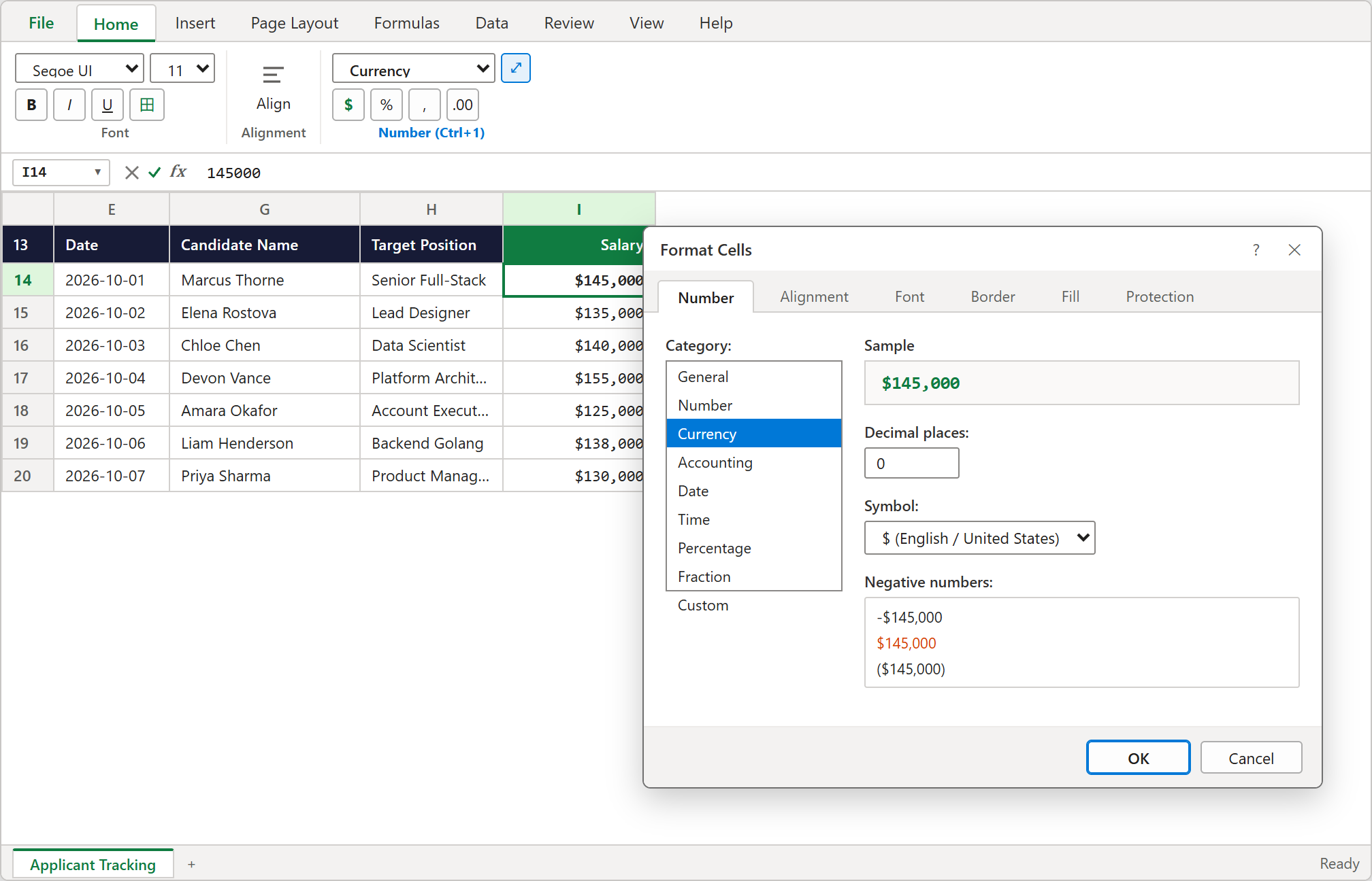
Figure 3: Format Cells dialog setting Currency to clean zero-decimal numbers with dollar signs.
Counting Applicants and Total Salary per Stage
Looking through individual applicants is helpful for recruiters, but department heads and finance leads usually want the big picture: how many people are in each stage, and how much payroll budget do we need if they accept?
Summing up column P in cell P20 shows our entire pipeline salary total of $2,248,000. Now let us showcase these numbers where leaders will see them immediately.
1Counting Applicants in Each Stage with COUNTIF
In cell O14, we use COUNTIF to count how many candidates in column F match the stage name written in cell N14.
Notice the dollar signs in $F$14:$F$30: they lock our search range in place so when you drag the formula down to row 19, Excel keeps checking the exact same candidate list without drifting.
2Summing Expected Salary per Stage with SUMIF
Candidate counts only tell half the story. Your finance partner also needs to know how much salary is tied up in each hiring stage so they can plan ahead for upcoming hires.
In column P, we use SUMIF to match candidates by their stage in column F and add up their salaries from column I. In cell P14, enter:
Building the Executive Header and Visual Charts
A good tracking sheet feels like a true dashboard when summary calculations connect directly into clear KPI cards and visual charts right at the top of your screen.
Your bar chart now neatly lists Sarah Jenkins at the top, perfectly matching the order of your recruiter summary table.
1Designing the Top Summary Banner
In rows 2 to 4, we set up a clean dark navy header (#171B36). Cells D2:J4 hold our dashboard title, while cards on the right display our two most important numbers.
The first card displays TOTAL ACTIVE POOL (17 Candidates in cell K3). The second card displays TOTAL PIPELINE SALARY, dynamically linked in cell N3 with =P20 so it always mirrors our $2,248,000 pipeline total.
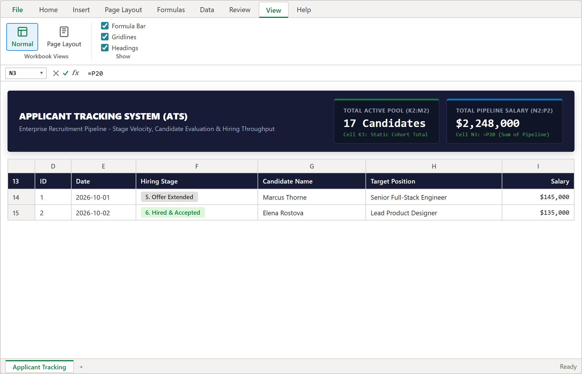
Figure 4: Executive header banner in rows 2 to 4 matching workbook.xlsx: Title block in D2:J4, Total Active Pool card in K2:M4, and Total Pipeline Salary card in N2:P4 linked to =P20.
2Adding the Pipeline Doughnut Chart
A doughnut chart gives everyone a quick visual sense of how applicants are moving through the funnel, showing whether candidates are stalling in early screens or progressing steadily toward offers.
Highlight our stage summary in cells N13:O19, switch to the Insert tab on the Ribbon, click Insert Pie or Doughnut Chart, and pick Doughnut.
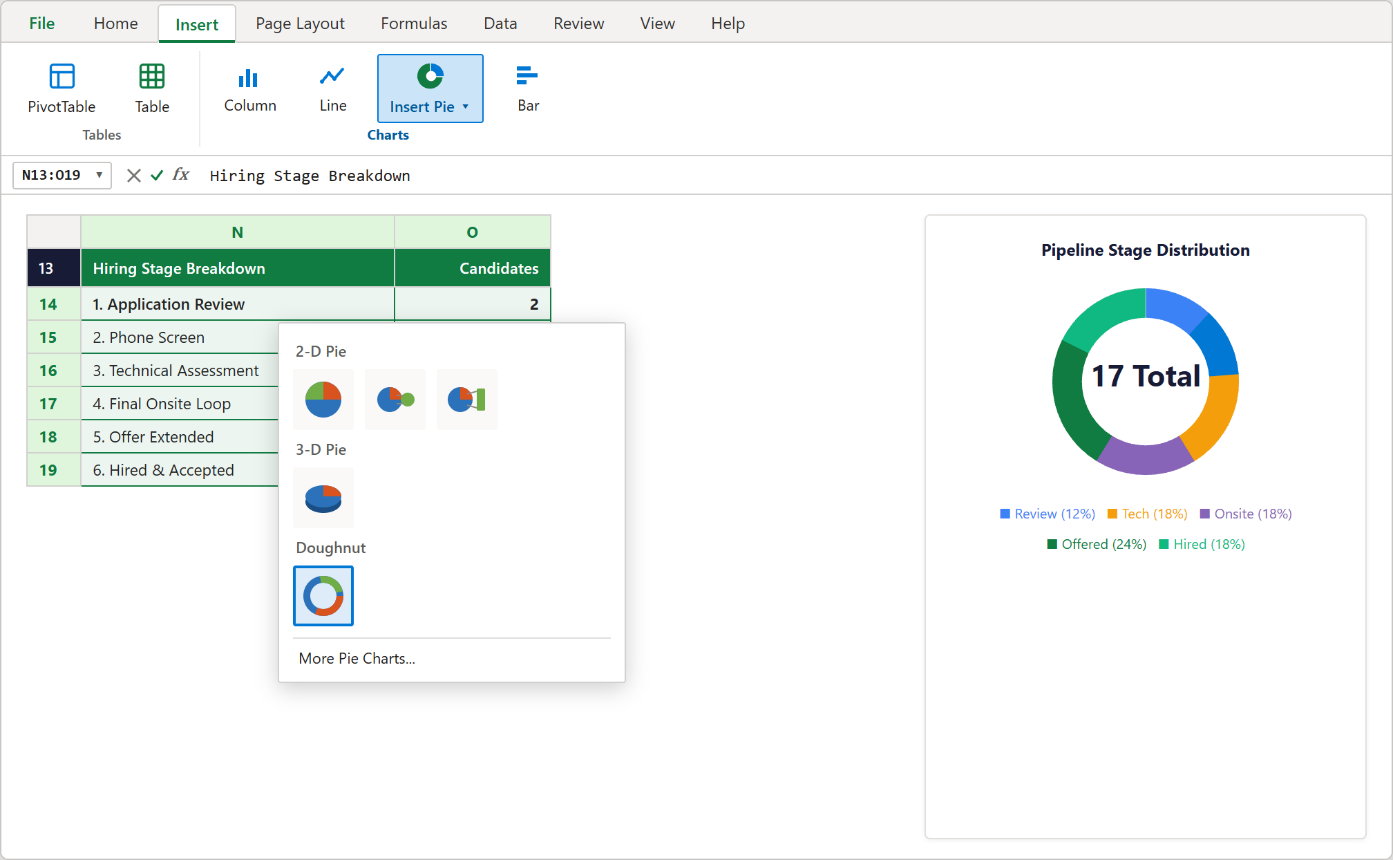
Figure 5: Selecting Insert > Doughnut Chart from the Excel Ribbon with stage summary data selected.
3Fixing the Recruiter Bar Chart Order
To see how many offers each recruiter has extended, select range N22:P28 and insert a 2-D Clustered Bar chart.
By default, Excel likes to list categories backwards from bottom to top, placing your first recruiter at the bottom. To fix this, double-click the vertical axis to open the Format Axis pane on the right, expand Axis Options, and check Categories in reverse order.
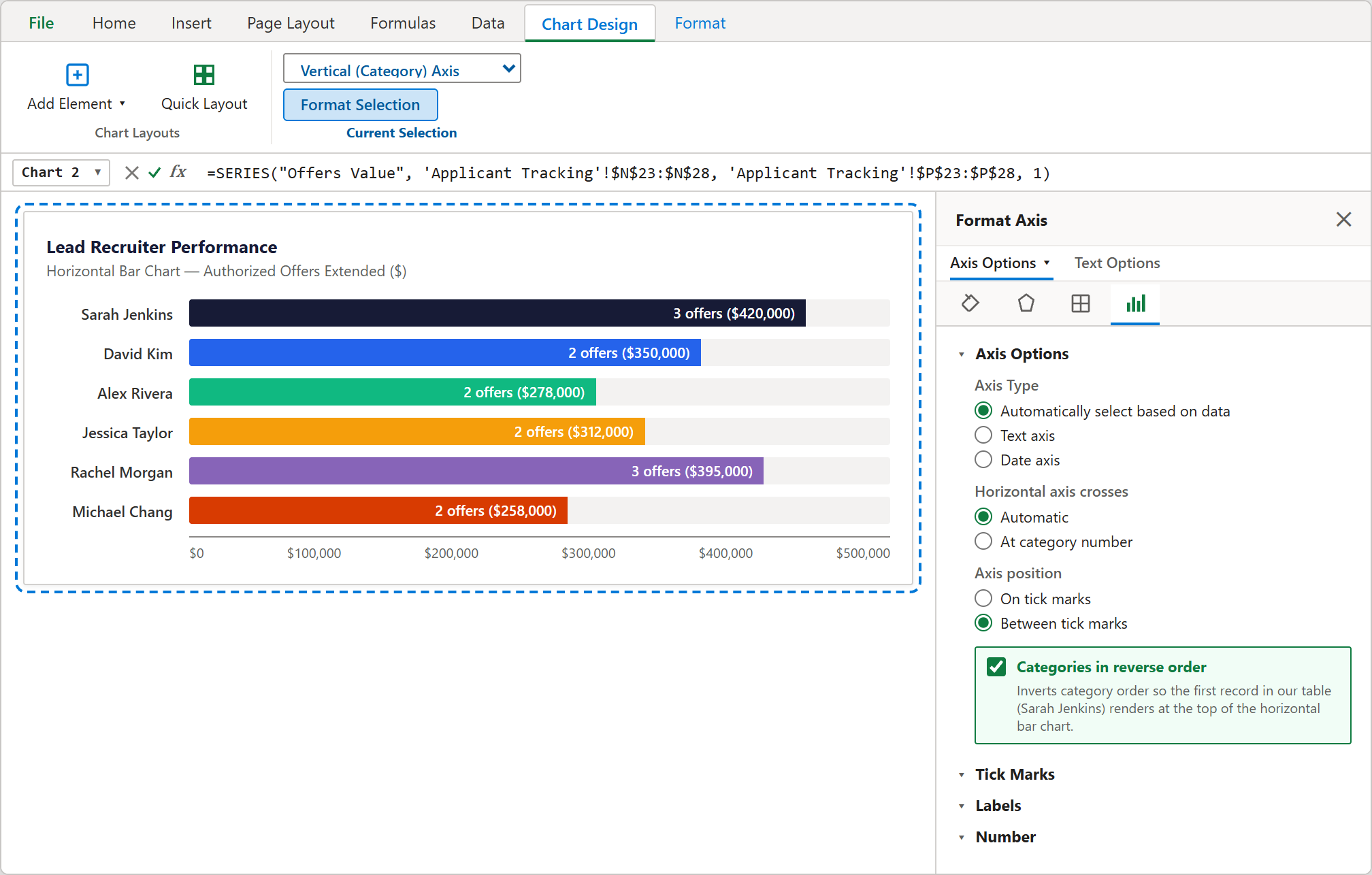
Figure 6: Checking Categories in reverse order in the Format Axis pane so recruiters appear in clean top-to-bottom order.
Conclusion
You now have a clean, automated Applicant Tracking System (ATS) in Microsoft Excel that your entire recruiting team can rely on every single day.
With stage dropdowns preventing typos, automatic scorecard checks handling offer approvals, and dynamic formulas keeping summary charts up to date, you will never have to spend hours cleaning up hiring numbers before a leadership meeting again.
During your weekly standups, simply update candidate stages in column F and log interview ratings in column K. All headcount summaries, recruiter charts, and pipeline totals will update automatically.
Download the completed workbook below to see all the working formulas in action, or test changes directly inside our interactive spreadsheet playground.

Spreadsheet educator and web developer passionate about hands-on interactive spreadsheet practice.
Related Practical Exercises
Explore more hands-on spreadsheet models with downloadable practice workbooks.
 Sales
Sales Commission Calculator Excel Template
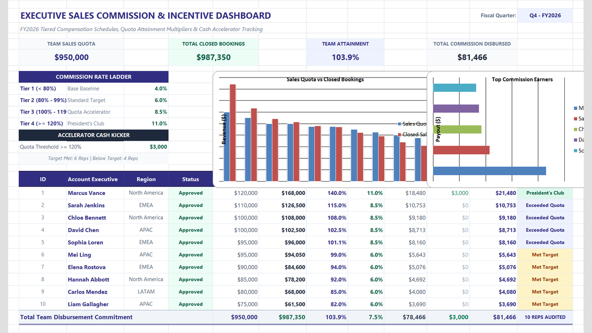
Calculate sales team commissions, quota attainment tiers, and performance accelerators in Microsoft Excel. Build an executive commission dashboard featuring tiered percentage multipliers, cash kickers for overachievers, automated performance status badges, and team payroll rollups.
 Sales
Sales Rep Performance Tracker Excel Template
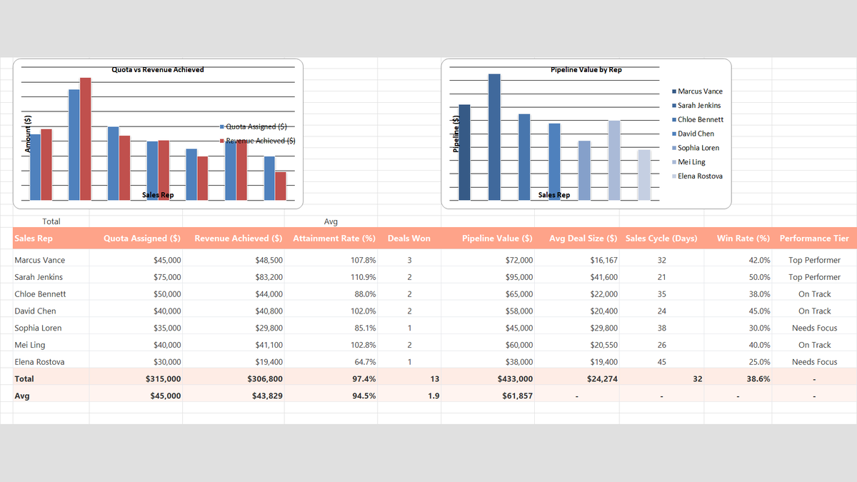
Build a practical sales rep performance tracker in Microsoft Excel to measure individual quota attainment, average deal size, win rates, and team pipeline velocity.
 Sales
Sales Pipeline Tracker Excel Template
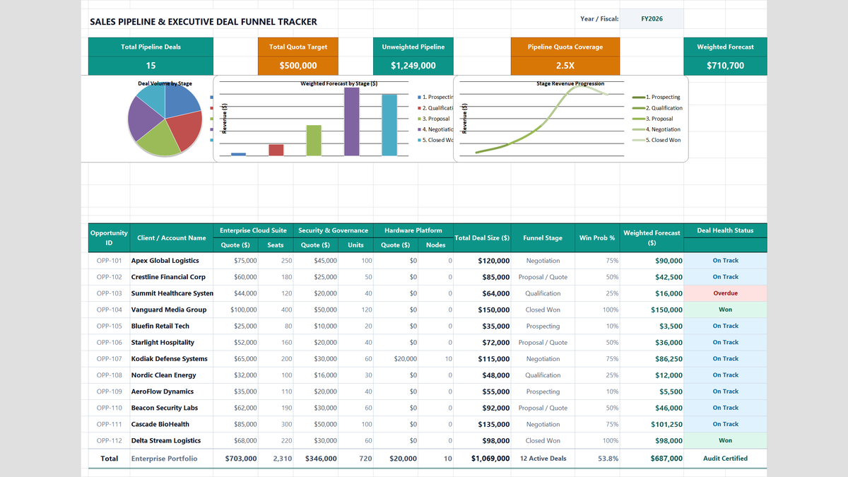
Learn how to construct an enterprise B2B sales pipeline tracker in Microsoft Excel featuring multi-product cross-sell quotes, weighted expected value forecasting, quota coverage ratios, and funnel conversion rollups.
 Finance
Product Pricing Calculator Excel Template
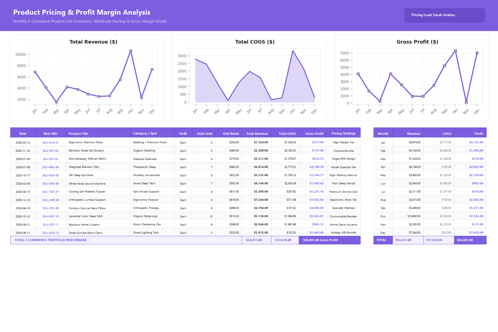
Build a practical product pricing and profit margin calculator in Microsoft Excel to track unit revenue, cost of goods sold, and monthly SKU profitability.
 Productivity
Student Gradebook GPA Calculator Excel Template
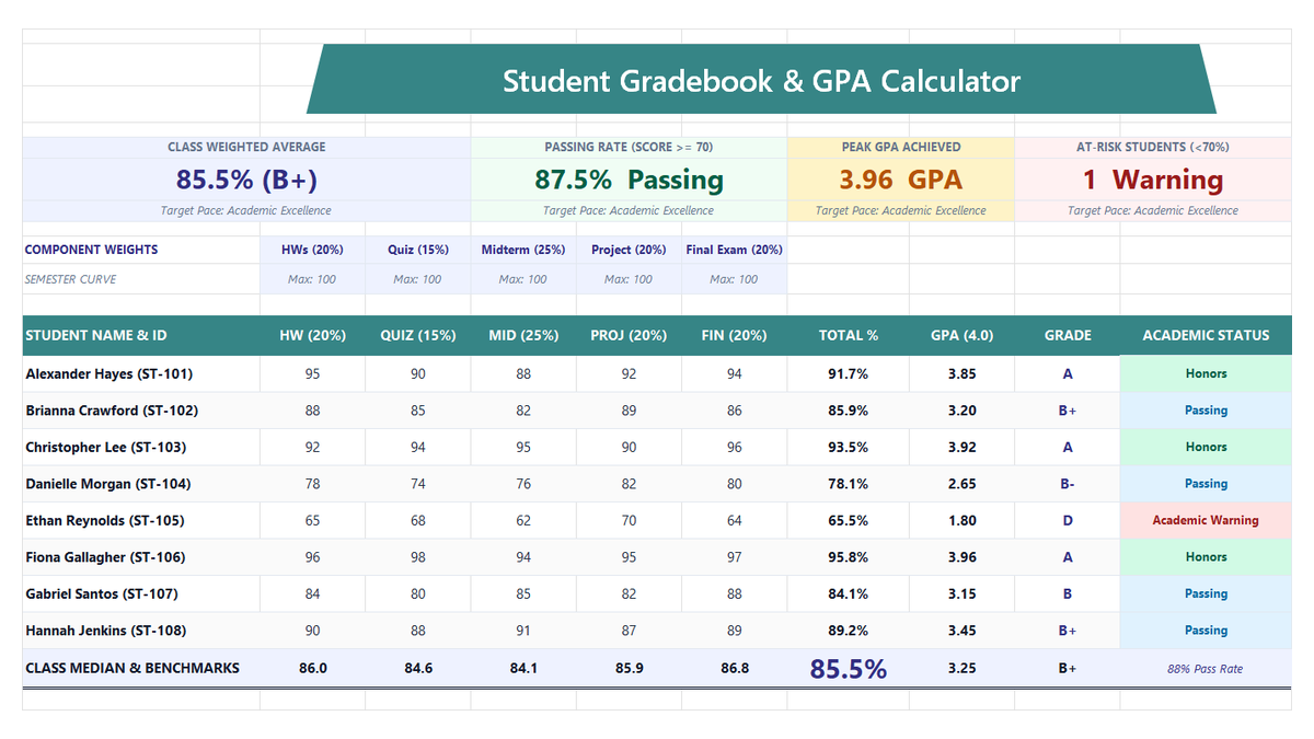
Build a practical student gradebook and semester GPA calculator in Microsoft Excel to compute weighted course grades, letter conversions, and class performance benchmarks.
Discussion
Ask questions, share formula tips, or discuss alternative approaches with fellow spreadsheet builders.
Loading discussion...