Picture a small software company in January. Three new customers each pay $36,000 up front for a full year of service, and the bank balance jumps by $108,000. The founder smiles, refreshes the banking app twice, and starts planning a team lunch.
Here is what the bank balance does not show. Each of those customers earns the company only $3,000 a month, so January revenue from them is $9,000, not $108,000. Meanwhile the cloud servers, the support team and the payroll keep sending bills every single month. A Profit and Loss statement, also called an income statement, lines up the revenue you earned with the costs it took to earn it. In this guide you will build a 12-month version in Excel, one step at a time.
Why Cash in the Bank Can Fool You
How the Workbook Is Laid Out
| Cell Range | Line Item Name | Item Category | Format | Business Role |
|---|---|---|---|---|
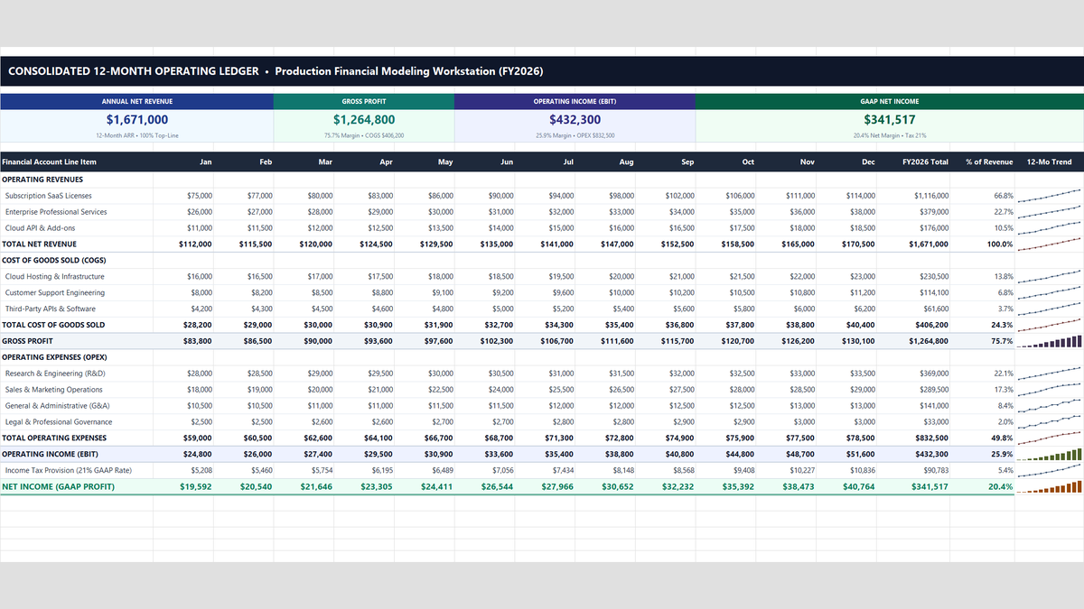
| B5, E5, H5, L5 | KPI Cards | Links to Totals | Number ($#,##0) | Point at O13, O19, O26 and O28. They show $1,671,000 revenue, $1,264,800 gross profit, $432,300 operating income and $341,517 net income. The small lines in row 6 are typed text. |
| C10:N12 | Operating Revenues | Monthly Inputs | Number ($#,##0) | Subscription SaaS licenses (row 10), enterprise professional services (row 11) and cloud API and add-ons (row 12). |
| C13:N13 | Total Net Revenue | Formula | Number ($#,##0) | Adds the three revenue streams with SUM. January is $112,000. |
| C15:N17 | Cost of Goods Sold (COGS) | Monthly Inputs | Number ($#,##0) | Direct delivery costs: cloud hosting (row 15), customer support engineering (row 16) and third-party APIs and software (row 17). |
| C18:N18 | Total Cost of Goods Sold | Formula | Number ($#,##0) | Adds rows 15 to 17. January is $28,200. |
| C19:N19 | Gross Profit | Formula | Number ($#,##0) | Revenue minus COGS (C13 minus C18). January is $83,800, a 74.8% gross margin. |
| C21:N24 | Operating Expenses (OPEX) | Monthly Inputs | Number ($#,##0) | Research and engineering (row 21), sales and marketing (row 22), general and administrative (row 23) and legal and professional governance (row 24). |
| C25:N25 | Total Operating Expenses | Formula | Number ($#,##0) | Adds rows 21 to 24. January is $59,000. |
| C26:N26 | Operating Income (EBIT) | Formula | Number ($#,##0) | Gross profit minus total OPEX (C19 minus C25). January is $24,800. |
| C27:N27 | Income Tax Provision (21%) | Formula | Number ($#,##0) | Operating income times 21%, rounded to whole dollars. January is $5,208. |
| C28:N28 | Net Income (GAAP Profit) | Formula | Number ($#,##0) | Operating income minus the tax provision (C26 minus C27). January is $19,592, closed with a top line and a double underline. |
| O10:O28 | FY2026 Total | Formula | Number ($#,##0) | Adds January to December for each line. Gross profit and operating income in column O are subtractions, so they match the monthly math. |
| P10:P28 | % of Revenue | Formula | Percentage (0.0%) | Each yearly total divided by O13, the yearly revenue total. Gross profit is 75.7% and net income is 20.4%. |
| Q10:Q28 | 12-Mo Trend | Sparklines | In-cell chart | One small chart per row, built from the twelve monthly values in columns C to N. |
With the map in hand, let us build the statement from the top down.
Build Your Profit and Loss Statement in Five Steps
1Step 1: Build Total Revenue and Gross Profit
Start with the money coming in. Type monthly revenue for subscriptions, professional services and API add-ons in rows 10 to 12. In row 13, use SUM to add the three streams. For January that gives $112,000.
Next, enter your direct delivery costs in rows 15 to 17: hosting, customer support and third-party software. Add them up in row 18, which gives $28,200 for January.
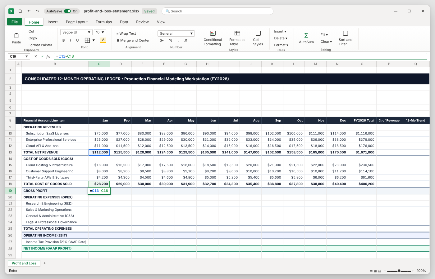
Now click C19. Build Gross Profit by taking total revenue (C13) and subtracting total COGS (C18). Click the two cells while you type, and Excel draws a colored box around each one. Press Enter, then drag the fill handle across to column N.
January ends at $83,800, a 74.8% gross margin. In plain words, about 75 cents of every dollar is left to pay for everything else.
2Step 2: Add Up Your Operating Expenses
Operating expenses (OPEX) are the costs of running the company, whether or not one more customer signs. Enter them by team in rows 21 to 24: research and engineering, sales and marketing, general and administrative, and legal.
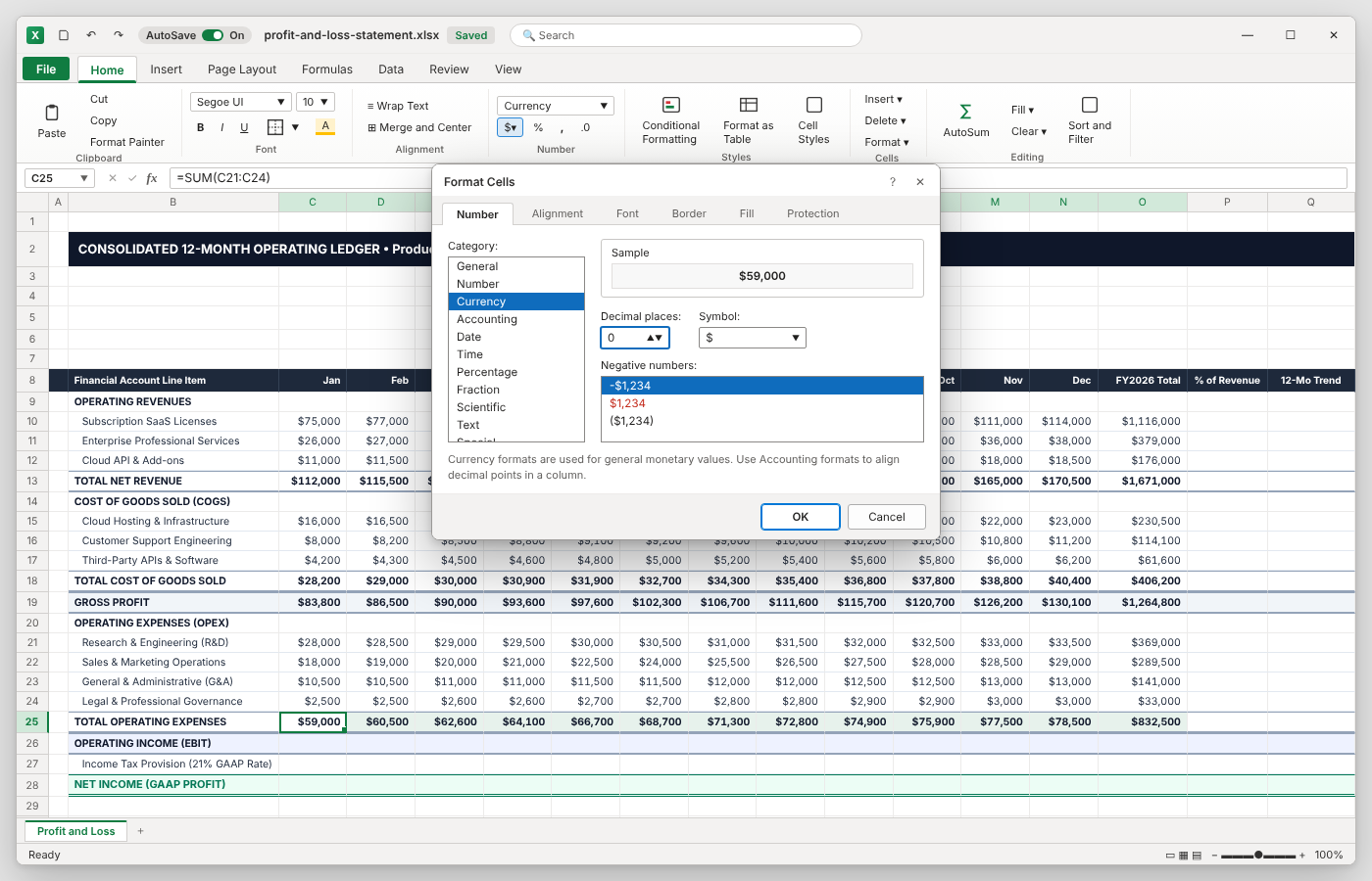
In C25, use SUM on the four cells right above it (C21 to C24), then fill it across to column N. January comes to $59,000.
Select C25:O25 and press Ctrl+1 to open Format Cells. On the Number tab, pick Currency, set Decimal places to 0 and keep the $ symbol. Make the row bold so totals stand out from inputs.
Why a range and not four cells joined with plus signs? If you insert a new row for insurance between rows 21 and 24, the range grows by itself. Insert inside the range, not below row 24, or Excel will not include it.
3Step 3: Find Operating Income and Net Income
Now for the two lines everyone asks about. Operating Income, often called EBIT (earnings before interest and taxes), goes in row 26. Take Gross Profit from row 19 and subtract Total Operating Expenses from row 25. January leaves $24,800.
Row 27 estimates tax at 21% of operating income and wraps the result in ROUND so you get whole dollars: $5,208 for January. Row 28 is Net Income, which is operating income minus that tax: $19,592.
In this template the 21% sits inside each formula. In your own model, type the rate in its own cell and point to it.
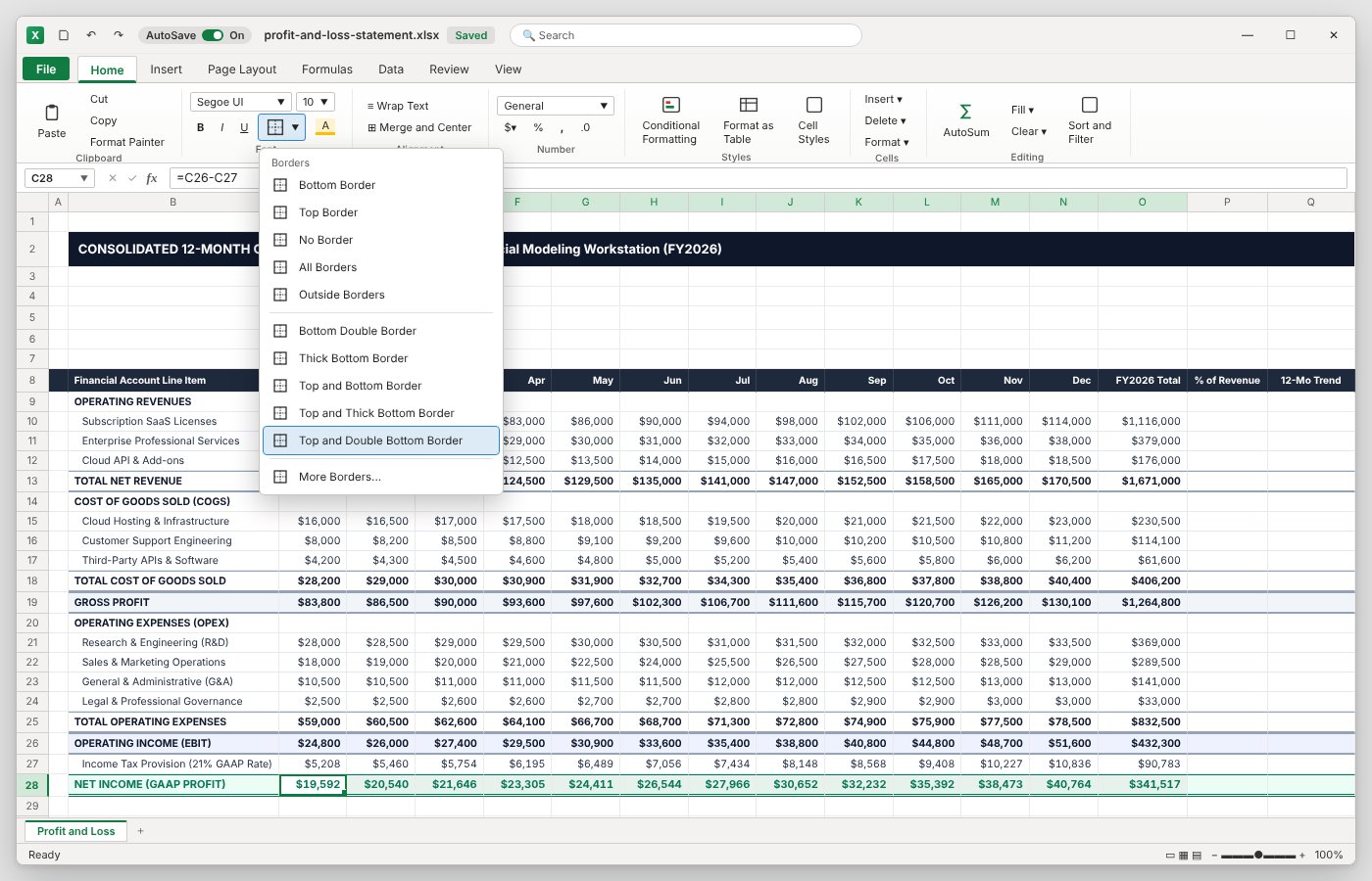
Finish by selecting C28:O28 and choosing Top and Double Bottom Border from the Borders menu on the Home tab. Accountants read that double line as the end of the statement.
4Step 4: Add a Percent of Revenue Column
Dollar amounts alone do not say whether a cost is getting out of hand. A percent-of-revenue column fixes that. In column P, divide each yearly total in column O by total revenue in O13. For Gross Profit, that means O19 divided by O13.
Add dollar signs to the revenue cell so it reads $O$13. They lock the reference, so it stays on O13 when you copy the formula down. Then format column P as Percentage with one decimal place.
Now the story is easy to see: direct costs take 24.3% of revenue, sales and marketing takes 17.3%, and net income is 20.4%.
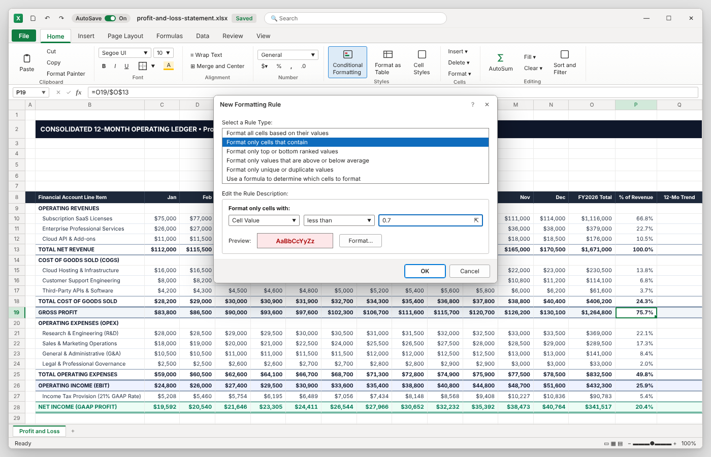
For an optional alert, select P19 and open Home > Conditional Formatting > New Rule. Choose Format only cells that contain, set Cell Value to less than 0.7, and pick a light red fill. The cell turns red if gross margin falls below a 70% target.
5Step 5: Connect the KPI Cards and Add Sparklines
Last, make the top zone useful. Link each big card number to its yearly total: B5 to O13, E5 to O19, H5 to O26 and L5 to O28. Now the cards change whenever the ledger changes.
The small lines under the numbers (row 6) are typed text here. To make them update too, build them with TEXT and cell references.
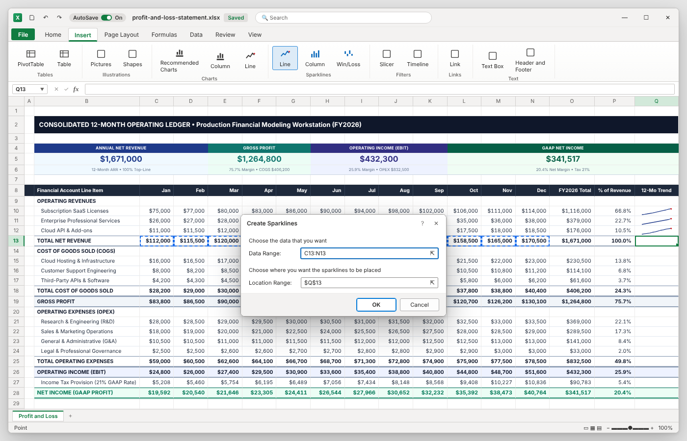
Then add the trend column. Select Q13 and go to Insert > Sparklines > Line. Set Data Range to C13:N13 and keep $Q$13 as the Location Range, then click OK. Repeat for the other rows you want to track. The preview uses column sparklines for the profit rows, which make month-to-month comparisons easier.
Wrap-Up and Template Download
Profit and Loss Statement Template Workbook
Microsoft Excel (.xlsx) • Production Model
Choose From 5 Specialized Template Variations
Download the exact layout built for your specific business model.
Multi-Step Corporate P&L
Includes Gross Profit, EBITDA, EBIT, EBT and Net Income tiers.
Simple Small Business P&L
Single-step layout (Income minus Expenses) for consultants and solo creators.
Comparative Quarterly P&L
Side-by-side Q1–Q4 quarterly performance tracked against annual budget variances.
SaaS & Subscription P&L
12-month cloud economics model with ARR, CAC marketing, and hosting COGS.
Restaurant & Retail P&L
Includes beginning/ending inventory calculations, food waste, and Prime Cost.

Spreadsheet educator and web developer passionate about hands-on interactive spreadsheet practice.
Related Practical Exercises
Explore more hands-on spreadsheet models with downloadable practice workbooks.
 Project Management
Project Budget Estimator Excel Template
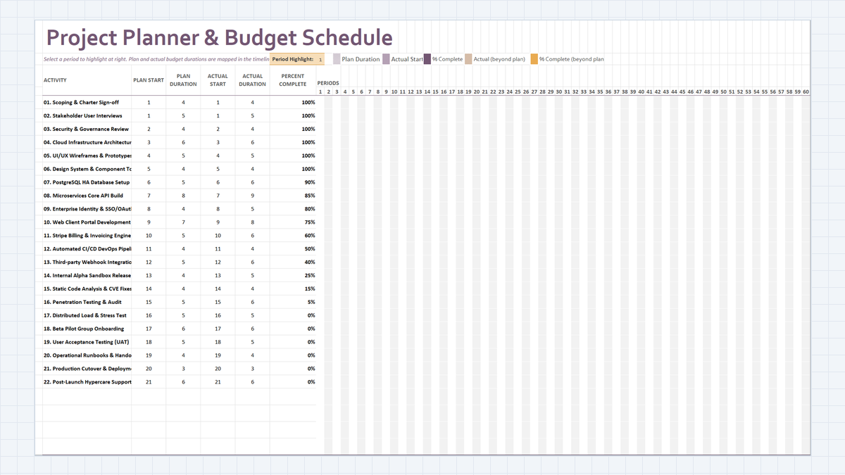
Build a Project Planner & Budget Schedule in Excel: 22 delivery workstreams, plan vs actual duration math, a dynamic in-cell Gantt chart, and percent-complete tracking that shows where schedule slippage starts.
 Project Management
Project Risk Register Excel Template
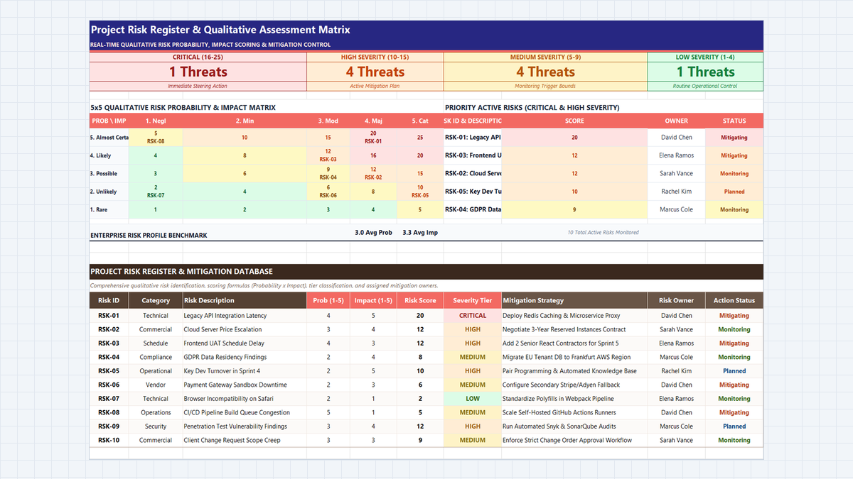
Learn enterprise risk governance in Microsoft Excel. Build an ISO 31000 and PMBOK-compliant 5x5 qualitative risk heatmap, automate probability and impact scoring, engineer multi-tier severity formulas, and enforce accountability with data validation.
 Operations
Purchase Order Tracker Excel Template
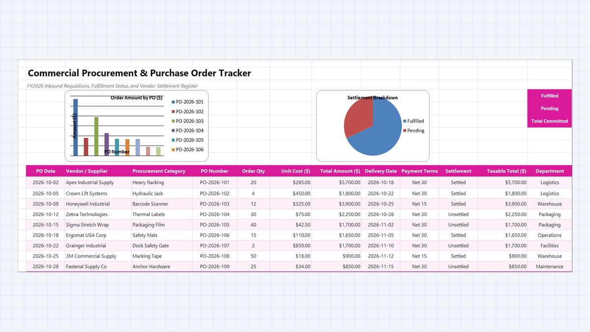
Learn how to engineer a commercial procurement and purchase order tracker in Microsoft Excel featuring line item commitment multiplication, vendor fulfillment status monitoring, and accounts payable settlement reconciliations.
 Operations
Vendor Performance Scorecard Excel Template
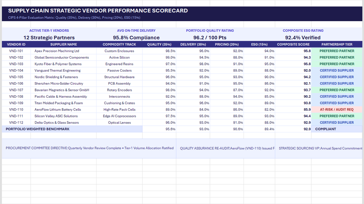
Learn strategic vendor evaluation in Microsoft Excel. Build a CIPS-compliant 4-pillar scorecard weighting Quality (35%), Delivery (30%), Pricing (20%), and ESG (15%). Automate weighted composite scores with SUMPRODUCT, calculate portfolio OTIF delivery, and establish tier-based purchase order allocations.
 Human Resources
Employee Timesheet Calculator Excel Template
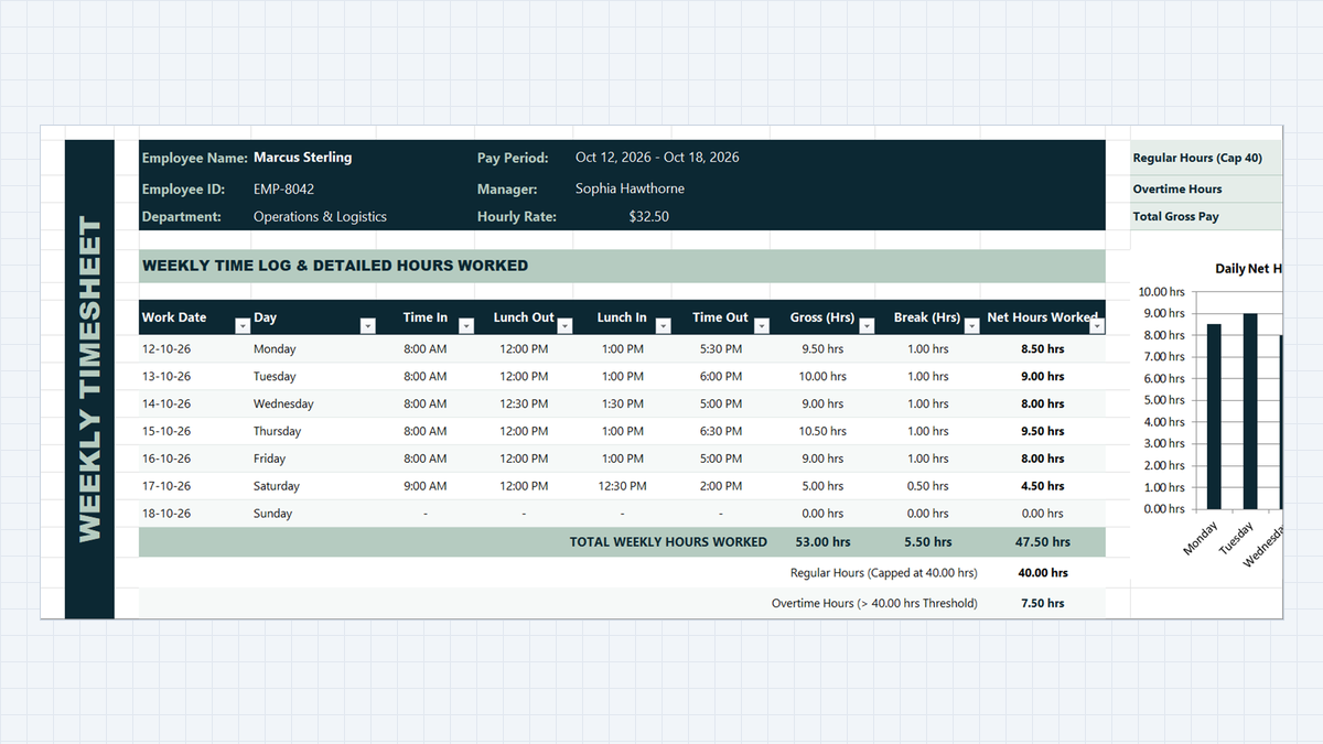
Track weekly employee work hours, lunch breaks, and overtime without mathematical headaches. Build a clean timesheet calculator in Microsoft Excel using simple time formulas, night-shift handling with MOD, and automatic overtime flags.
Discussion
Ask questions, share formula tips, or discuss alternative approaches with fellow spreadsheet builders.
Loading discussion...