Picture this. Your P&L says the business earned $220,000 this year, yet the finance director still can't explain the bank balance. If that sounds familiar, you need a 12-Month Cash Flow Statement Excel Template, and this guide shows you how to build one.
Here is the catch: profit is an accounting opinion, while cash pays salaries on Friday. In our workbook the company earns $220,000, but its cash grows by only $140,000, from $250,000 to $390,000. We will follow every number so you can see where the other $80,000 went.
We use the GAAP indirect method, three simple sections and five practical steps. Open the workbook next to this page and follow along.
Why Profit Is Not the Same as Cash
Anatomy of the 12-Month Cash Flow Statement Excel Template
12-Month Cash Flow. Column B holds labels, columns C to N are January to December, and column O is the full-year total.| Col | Field | Type | Format | Role |
|---|---|---|---|---|
| B | Activity | Text | General | Line item. |
| C:N | Jan to Dec | Input or formula | $#,##0;($#,##0) | Monthly cash movement. |
| O | FY2026 Total | Formula | $#,##0;($#,##0) | <code>SUM</code> of the twelve months. |
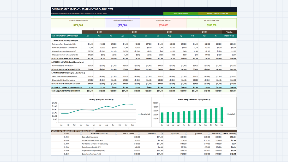
The finished workbook: cards on top, three sections in the middle, charts and ledger below.
Two design choices keep this Corporate Treasury Model simple. Every outflow is a negative number, so each total is plain addition. And the Ending Cash row is a bridge: each month starts from last month's closing balance. One note on M3: the 14.8-month runway is typed text, not a formula, so update it by hand.
5 Steps to Build It in Excel
1Step 1: Set Up the Three Sections and Accounting Format
Type the three headings in column B: 1. OPERATING ACTIVITIES in row 11, 2. INVESTING ACTIVITIES in row 17 and 3. FINANCING ACTIVITIES in row 20. Enter the monthly inputs under them. Raw numbers like -2500 are hard to read, so format them next.
Select C12:O25, press Ctrl+1 and choose Accounting. Set decimal places to 0 and the symbol to $. Negatives now sit in brackets, like (2,500). The template uses the custom code "$"#,##0;("$"#,##0);"-", which also shows a dash for zero.

Step 1: Format Cells with Accounting applied to C12:O25.
2Step 2: Build the Operating Cash Flow Engine
Click C16 and use AutoSum, or type =SUM(C12:C15). For January this adds net income ($15,000), the depreciation add-back ($2,800), the receivables change (($2,500)) and the inventory and payables change (($1,200)): $14,100.
Depreciation is added back because it lowered profit but never left your bank. Fill the formula across to N16, then set O16 to =SUM(C16:N16). The year lands at $256,500.

Step 2: C16 in edit mode with =SUM(C12:C15).
3Step 3: Calculate Free Cash Flow to Firm (FCFF)
Row 19 simply repeats row 18, so C19 is =C18. Link the cards next: B7 is =O16 and E7 is =O19. Then click H7, press F2 and type =B7+E7.
CapEx is already negative, so the result is $256,500 + ($62,500) = $194,000. This Free Cash Flow to Firm FCFF Excel figure is what lenders check first: the cash left after keeping your servers alive.

Step 3: H7 in edit mode with =B7+E7.
4Step 4: Roll the Cash Balance Forward
In C24 add the three sections: =C16+C19+C23. In C25 start from the opening balance: =250000+C24, which gives $257,100.
In D25 type =C25+D24. Select D25:N25 and press Ctrl+R (Fill Right). Every month now starts from the last closing balance, and December ends at $390,000. Set O25 to =N25 so the card in L7 can pick it up.

Step 4: Fill Right applied to D25:N25.
5Step 5: Add a Low-Cash Alert
Select C25:N25. Go to Home, then Conditional Formatting, then Highlight Cells Rules, then Less Than. Type 270000 as your safety buffer and pick Light Red Fill with Dark Red Text.
The $270,000 buffer is only our example. With it, January ($257,100), February ($262,800) and March ($268,000) turn red, so the first quarter clearly looks tightest. Pick a buffer from your own loan terms or payroll needs.

Step 5: Less Than rule with a 270,000 buffer.
Working Capital Traps: Why Fast Growth Can Drain Cash
Download the Template and Keep Going

Spreadsheet educator and web developer passionate about hands-on interactive spreadsheet practice.
Related Practical Exercises
Explore more hands-on spreadsheet models with downloadable practice workbooks.
 Human Resources
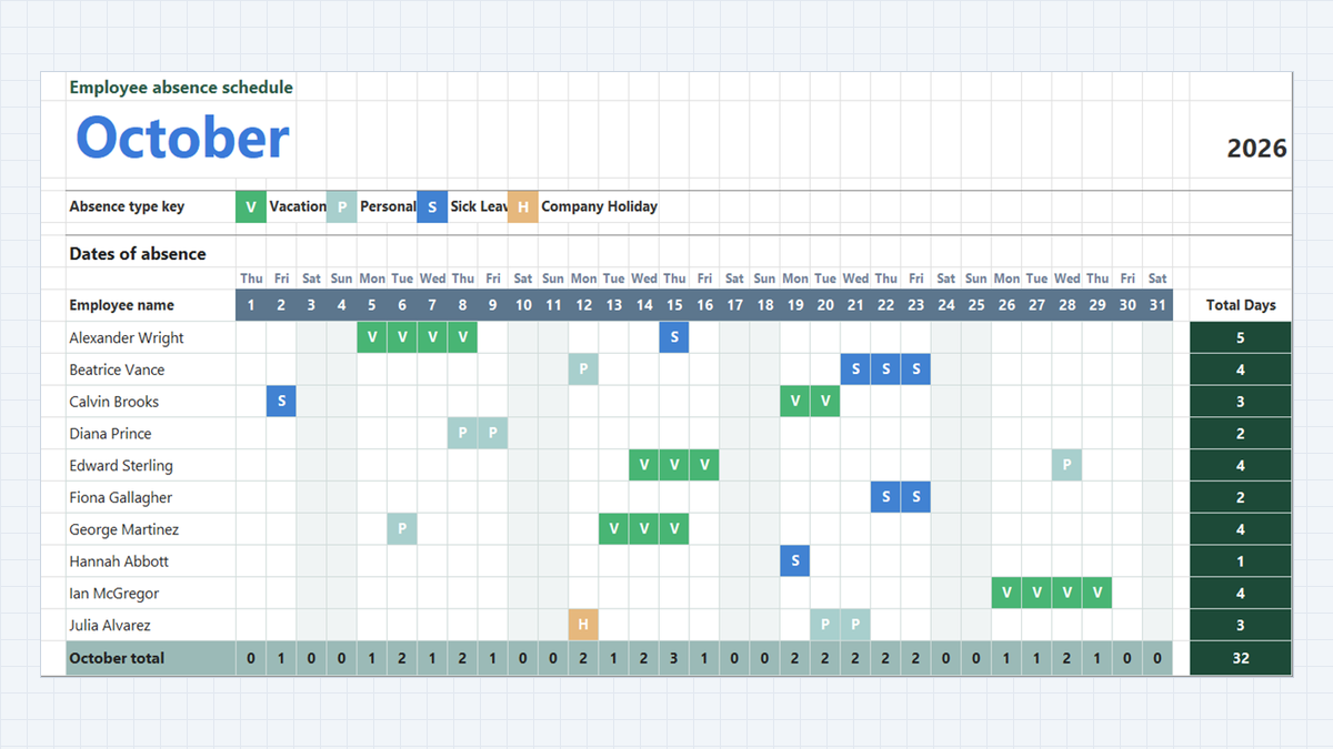
Employee Attendance Tracker Excel Template
Manage team attendance, vacation days, and sick leave in Microsoft Excel. Build a clean monthly absence schedule featuring dropdown absence keys with Data Validation, automatic color-coded badges via Conditional Formatting, and dynamic attendance totals with COUNTA.
 Human Resources
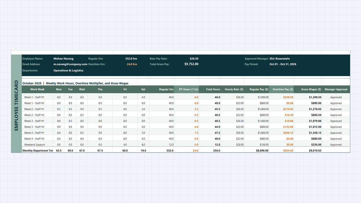
Employee Payroll Calculator Excel Template
Payroll Friday should not be stressful. Learn how to build an employee payroll calculator in Microsoft Excel that automatically tallies timecards, caps regular hours at 40 with MIN, computes 1.5x overtime with MAX, and locks penny-perfect wages with ROUND.
 Finance
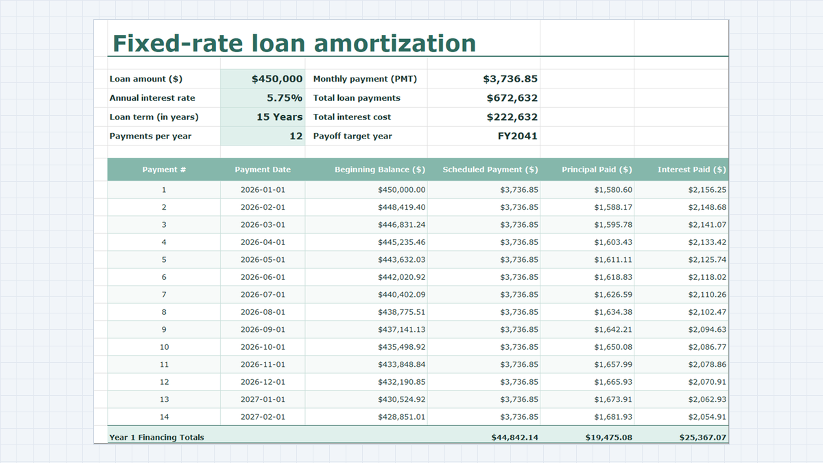
Loan Amortization Schedule Excel Template
Learn fixed-rate commercial debt structuring in Microsoft Excel. Build a rigorous amortization schedule featuring level debt service calculations with =PMT(), interest and principal bifurcation, dynamic balance rollforwards, accounting ledger formatting, and annual debt covenant rollups.
 Productivity
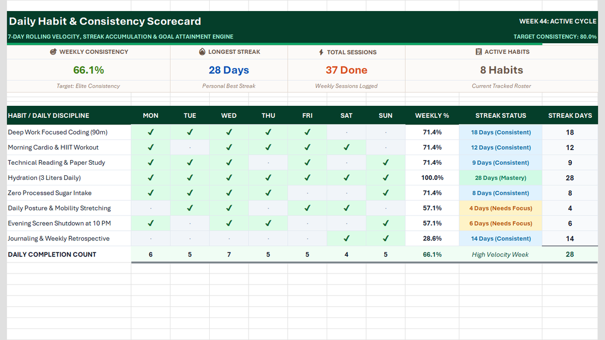
Daily Habit Tracker Excel Template
Build a Daily Habit Tracker in Excel: a 7-day grid of checkmarks and dots, COUNTIF completion rates, daily volume, streaks, and a four-card weekly scorecard.
 Productivity
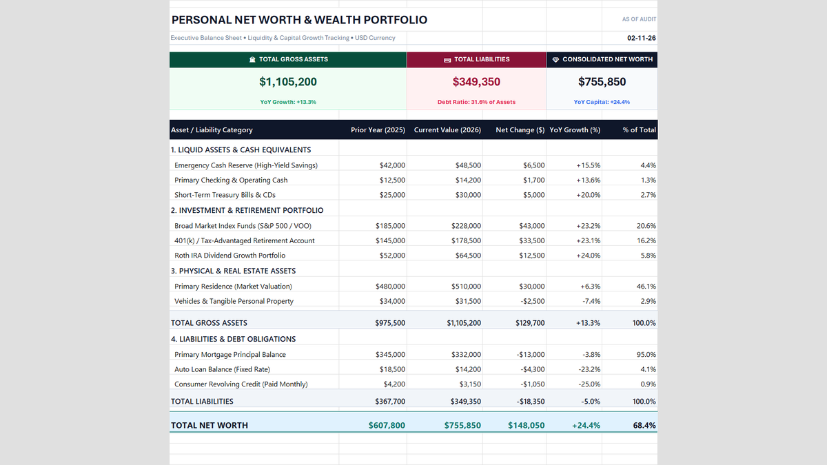
Personal Net Worth Tracker Excel Template
Build a personal net worth tracker in Excel that compares two years of liquid cash, investments, home equity and debt, then calculates net worth, year-over-year growth and allocation health with simple formulas.
Discussion
Ask questions, share formula tips, or discuss alternative approaches with fellow spreadsheet builders.
Loading discussion...