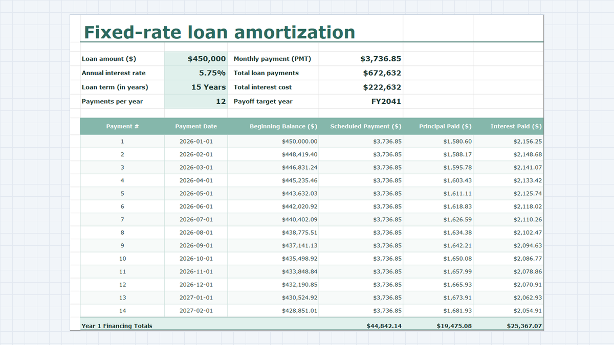
Commercial Debt Architecture & Underwriting Fundamentals
Facility Terms & Financial Ledger Data Dictionary
| Cell Range | Parameter / Metric Name | Data Type | Number Format | Description & Modeling Rule |
|---|---|---|---|---|
| C3 | Loan Amount (Principal PV) | Numeric Currency | Accounting ($#,##0) | Original principal commitment of the loan facility ($450,000.00). |
| C4 | Annual Interest Rate | Numeric Percentage | 0.00% | Contractual nominal annual coupon (5.75%). Must be divided by compounding frequency in periodic calculations. |
| C5 | Loan Term (Tenor) | Numeric Integer | General ("15 Years") | Overall facility duration in years (15 years = 180 monthly periods). |
| C6 | Payments Per Year | Numeric Integer | General | Annual payment frequency (12 for monthly payments). |
| E3 | Monthly Payment (Debt Service) | Formula Output | Accounting ($#,##0.00) | =PMT(C4/C6, C5*C6, -C3). Fixed monthly annuity payment ($3,736.85). |
| E4 | Total Payments | Formula Output | Accounting ($#,##0) | =E3*(C5*C6). Aggregate nominal cash outflow across the facility tenor ($672,632). |
| E5 | Total Interest | Formula Output | Accounting ($#,##0) | =E4-C3. Cumulative financing charge incurred by the borrower ($222,632). |
| B9:B22 | Payment Index (Pmt #) | Integer Sequence | Center Align | Sequential period counter running from 1 through the maturity period (180). |
| C9:C22 | Payment Date | Calendar Date | DD/MM/YYYY | Payment due date. Increments monthly via regular corporate settlement schedule. |
| D9:D22 | Beginning Balance | Formula Reference | Accounting ($#,##0.00) | Period opening liability. Period 1 links to =C3; period 2+ links to previous ending balance =H9. |
| E9:E22 | Scheduled Payment | Absolute Reference | Accounting ($#,##0.00) | Fixed monthly debt service linking to =$E$3 ($3,736.85). |
| F9:F22 | Principal Paid | Formula Calculation | Accounting ($#,##0.00) | =E9-G9. The portion of debt service that directly repays the debt liability. |
| G9:G22 | Interest Paid | Formula Calculation | Accounting ($#,##0.00) | =D9*(C$4/C$6). Period interest expense recognized on the opening principal balance. |
| H9:H22 | Ending Balance | Formula Calculation | Accounting ($#,##0.00) | =D9-F9. Closing outstanding loan principal at the end of the period. |
Step-by-Step Amortization Ledger Build
3.1Step 1: Calculating Level Debt Service with =PMT()
Excel provides the built-in financial function =PMT(rate, nper, pv, [fv], [type]) to determine the constant periodic annuity payment required to fully extinguish a loan balance. In corporate debt modeling, three critical rules govern its implementation:
First, the rate argument must represent the periodic interest rate, computed by dividing the annual coupon by annual payments: C4/C6 (5.75% / 12 = 0.479167% per month). Second, the nper argument represents total payment periods across the life of the loan: C5*C6 (15 years * 12 = 180 months). Third, the present value pv must be entered as a negative value -C3 (or the formula prefixed with a minus sign) so that the resulting debt service displays as a positive cash disbursement rather than a negative cash flow.
Select cell E3 and input the formula: =PMT(C4/C6, C5*C6, -C3). This yields an exact monthly debt service requirement of $3,736.85.
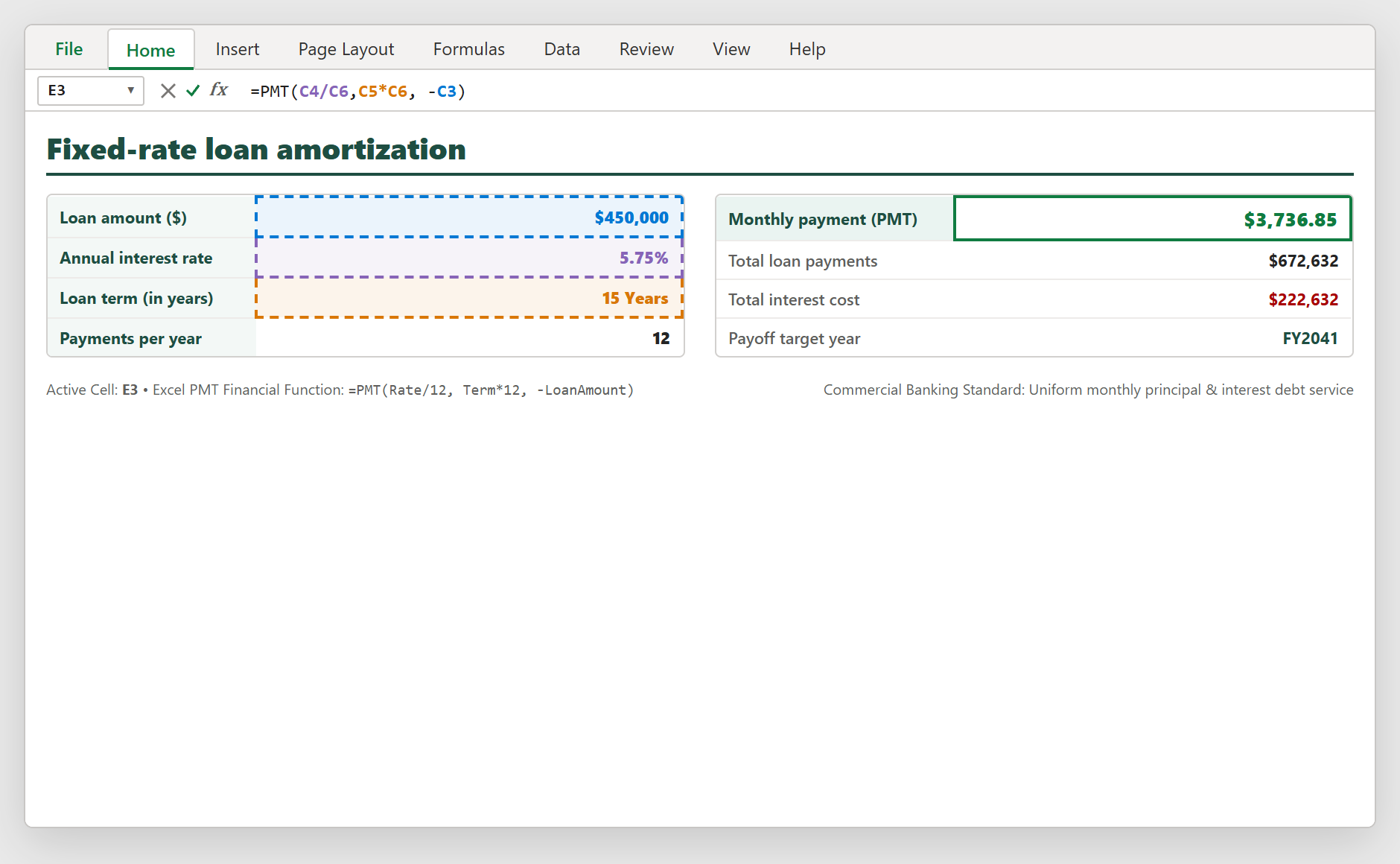
Figure 1: Executing the =PMT() annuity calculation in cell E3 with color-coded cell references for annual rate, tenor, and principal commitment.
3.2Step 2: Configuring Accounting Number Formatting
In financial ledgers, raw unformatted numbers look unpolished and obscure decimal variance. Corporate lending standards require the Accounting number format, which anchors currency symbols ($) flush against the left cell border, aligns decimal points vertically down the entire column, and displays zero balances cleanly as hyphens (-).
Highlight the entire schedule range D9:H22 along with summary cells C3 and E3:E5. Press Ctrl + 1 to open the Format Cells dialog box.
Under the Category menu on the left, select Accounting. Confirm that Decimal places is set to 2 and the Symbol dropdown is configured to $ ($). Click OK to apply. Notice how this immediately formats all monetary values into clean, institutional figures like $ 450,000.00 and $ 3,736.85.
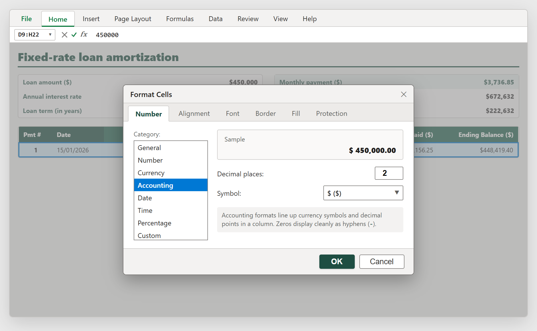
Figure 2: Configuring the official Accounting format via the Format Cells dialog (Ctrl + 1) to align currency columns and ensure zero-hyphen audit compliance.
3.3Step 3: Calculating Period Interest & Principal Paydown
Each fixed payment of $3,736.85 must be partitioned into its two constituent accounting components: interest expense (tax-deductible operational cost) and principal reduction (balance sheet liability repayment).
In Month 1 (Row 9), opening principal in D9 is $450,000.00. The accrued interest for the month is calculated by multiplying the opening balance by the monthly interest rate: =D9*(C$4/C$6). Notice the mixed cell references C$4 and C$6 with dollar signs locking the row number. This ensures that when the formula is copied down across 180 rows, the rate and payment frequency remain anchored to the header parameter block.
In cell G9, enter: =D9*(C$4/C$6) ($2,156.25). Once period interest is determined, the remaining portion of the fixed scheduled payment directly pays down loan principal in cell F9: =E9-G9 ($1,580.60). As principal decreases each month, subsequent interest charges shrink, shifting a progressively higher percentage of each fixed payment toward principal retirement.
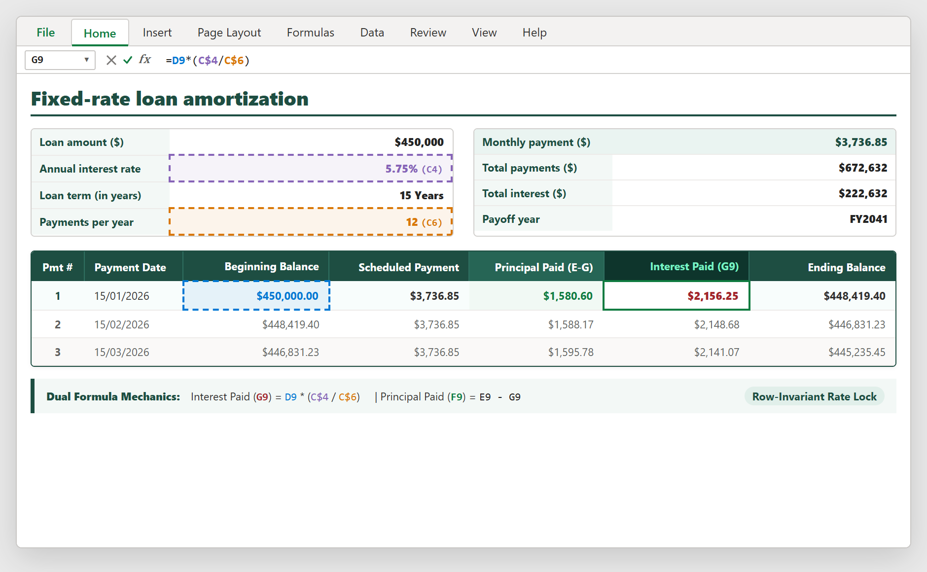
Figure 3: Formulating the interest-principal split in Period 1 using row-locked cell references (C$4 and C$6) for rate stability.
3.4Step 4: Engineering Unbroken Balance Rollforward Links
The core engine of any financial debt schedule is the balance rollforward: Ending Balance = Beginning Balance - Principal Paid.
In Month 1, cell H9 calculates: =D9-F9 ($450,000.00 - $1,580.60 = $448,419.40). For Month 2 (Row 10), the beginning balance must inherit the previous period closing balance. Never hardcode or re-enter balances manually. In cell D10, enter the dynamic reference: =H9.
This single relative reference establishes an unbroken mathematical chain. Once set, you can copy cells D10:H10 down through all 180 periods. Any unscheduled prepayments or interest rate adjustments automatically ripple across all remaining periods without manual intervention.
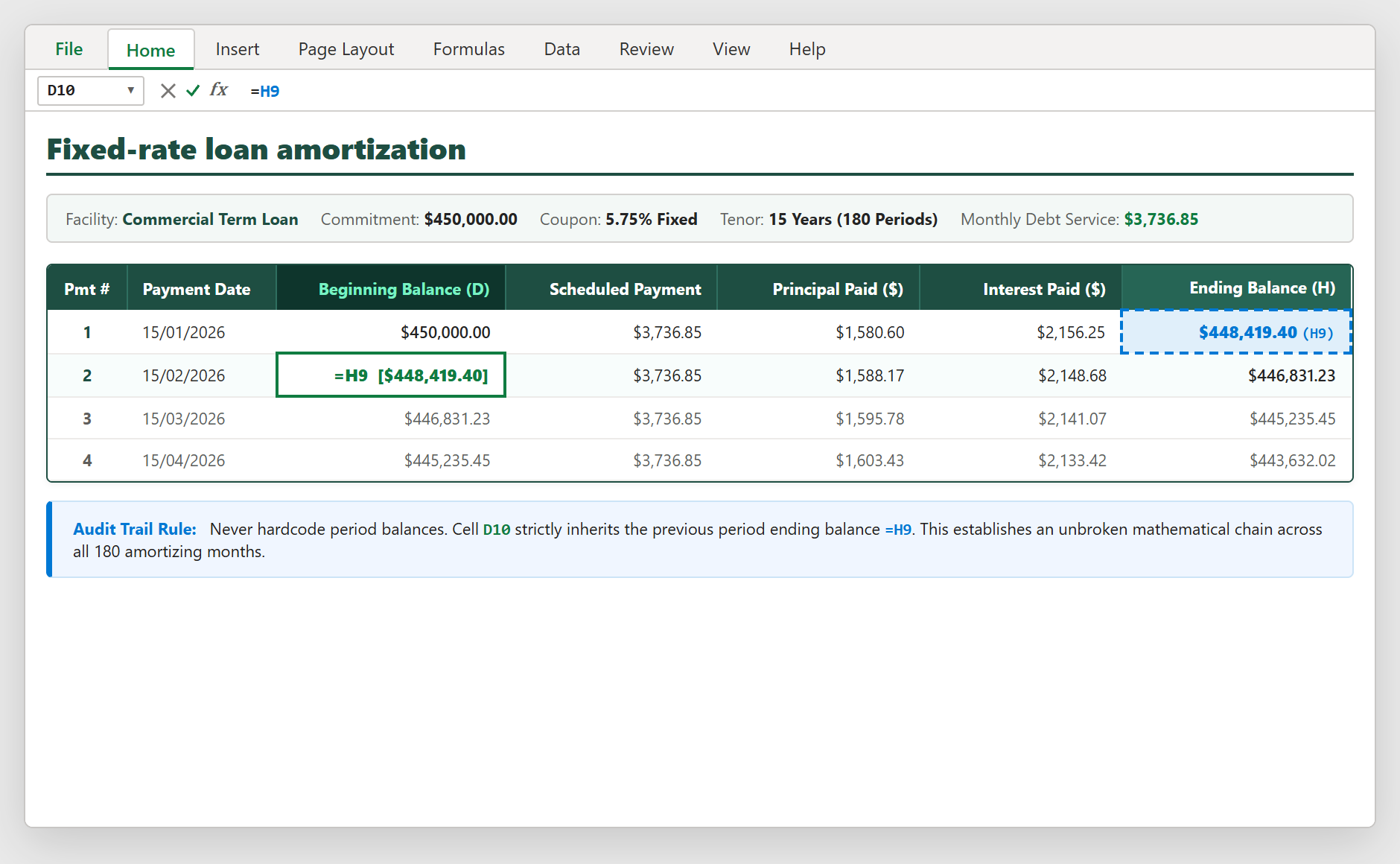
Figure 4: Dynamic balance rollforward linkage in cell D10 (=H9) connecting consecutive monthly amortization periods.
3.5Step 5: Aggregating Annual Debt Service Rollups
Corporate lenders and CFOs evaluate debt service on an annual basis to verify compliance with financial covenants. In Row 23, construct the Year 1 Financing Totals rollup row beneath Period 12.
For Scheduled Payments (cell E23), sum the 12 monthly payments: =SUM(E9:E22) ($44,842.20). For Principal Paid (cell F23), sum total principal retired: =SUM(F9:F22) ($19,475.01). For Interest Paid (cell G23), sum total financing charges: =SUM(G9:G22) ($25,367.19). For Ending Balance (cell H23), reference the final period closing balance: =H22 ($430,524.99).
Notice the mathematical verification: Scheduled Payments ($44,842.20) exactly equals Principal ($19,475.01) plus Interest ($25,367.19). In Year 1, interest represents 56.57% of all payments made, illustrating the front-loaded nature of long-term commercial loans.
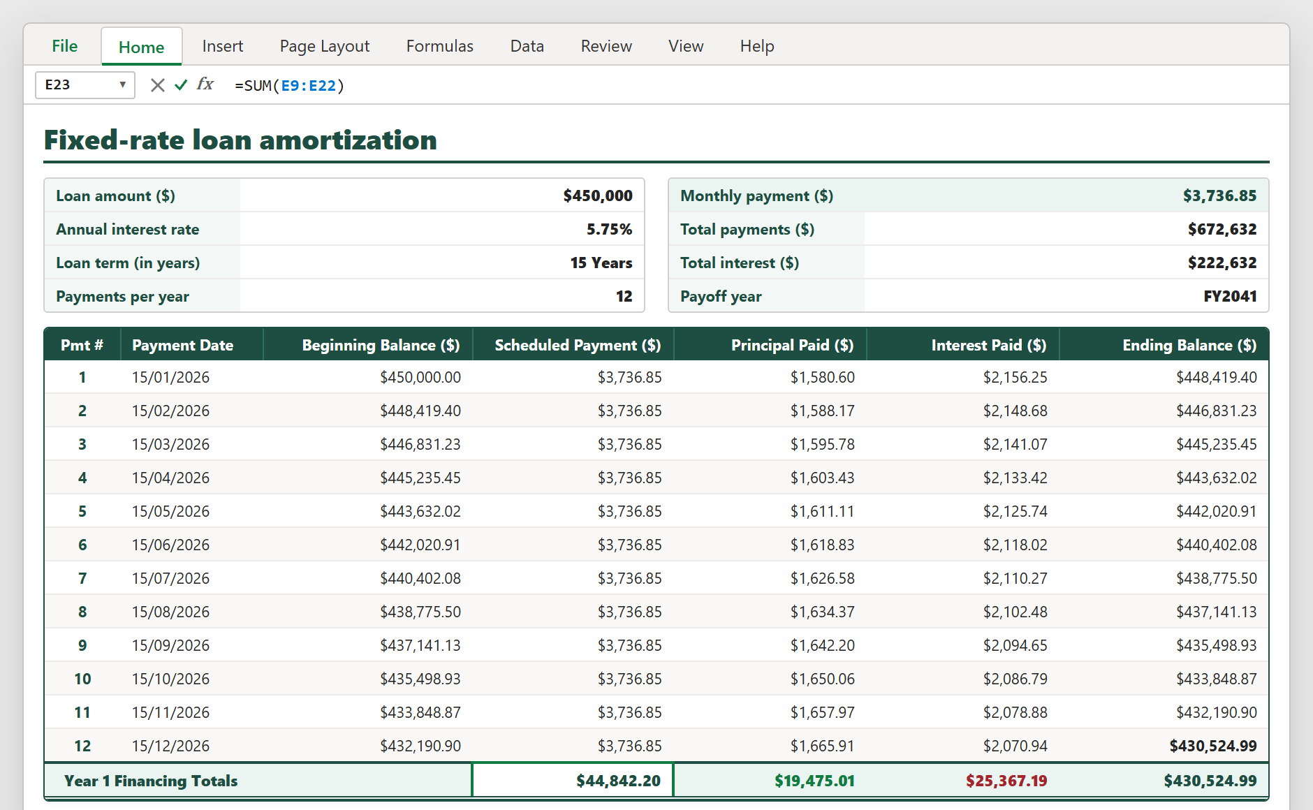
Figure 5: Complete Year 1 commercial loan amortization schedule showing monthly payment progression and year-end rollup totals.
Treasury Audit Checks, Covenants & Common Traps

Spreadsheet educator and web developer passionate about hands-on interactive spreadsheet practice.
Related Practical Exercises
Explore more hands-on spreadsheet models with downloadable practice workbooks.
 Productivity
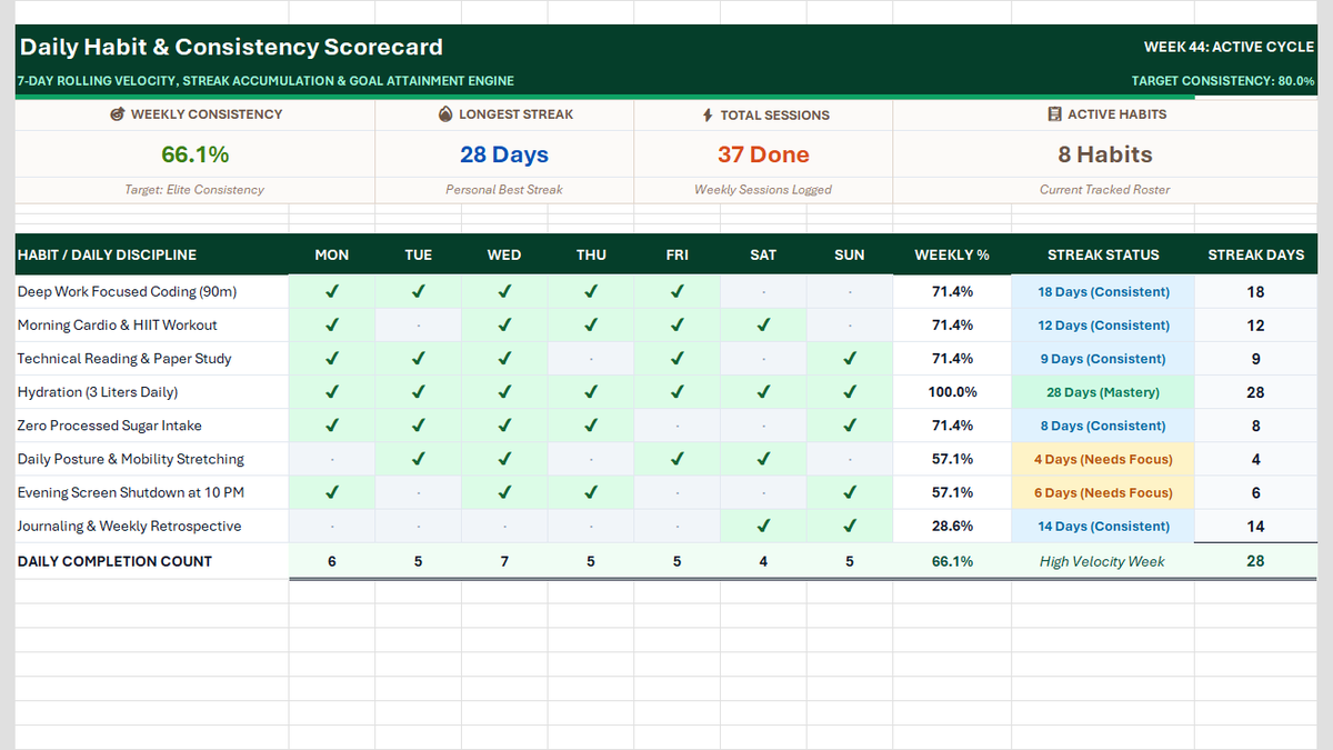
Daily Habit Tracker Excel Template
Build a Daily Habit Tracker in Excel: a 7-day grid of checkmarks and dots, COUNTIF completion rates, daily volume, streaks, and a four-card weekly scorecard.
 Productivity
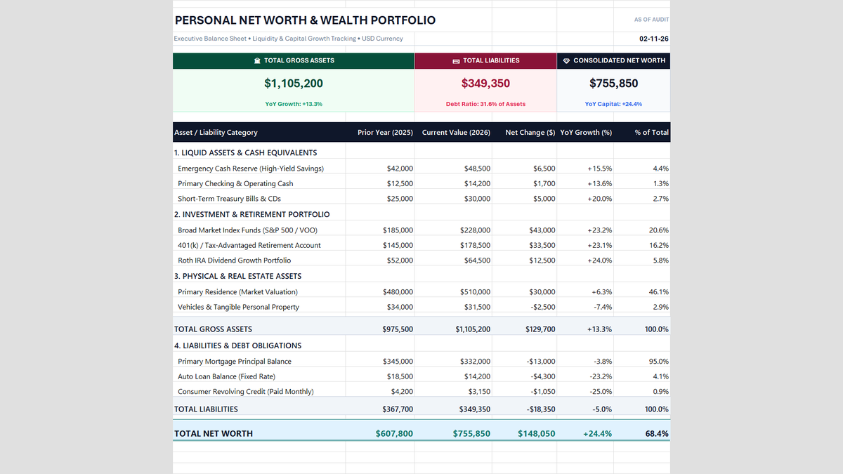
Personal Net Worth Tracker Excel Template
Build a personal net worth tracker in Excel that compares two years of liquid cash, investments, home equity and debt, then calculates net worth, year-over-year growth and allocation health with simple formulas.
 Finance
Profit and Loss Statement Template
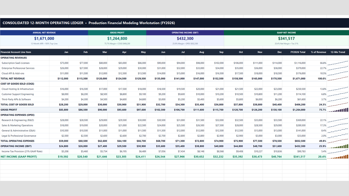
A 12-month Profit and Loss statement in Excel that shows where every revenue dollar goes. Type your monthly numbers once, and gross profit, operating income, tax, net income and margin percentages update on their own.
 Project Management
Project Budget Estimator Excel Template
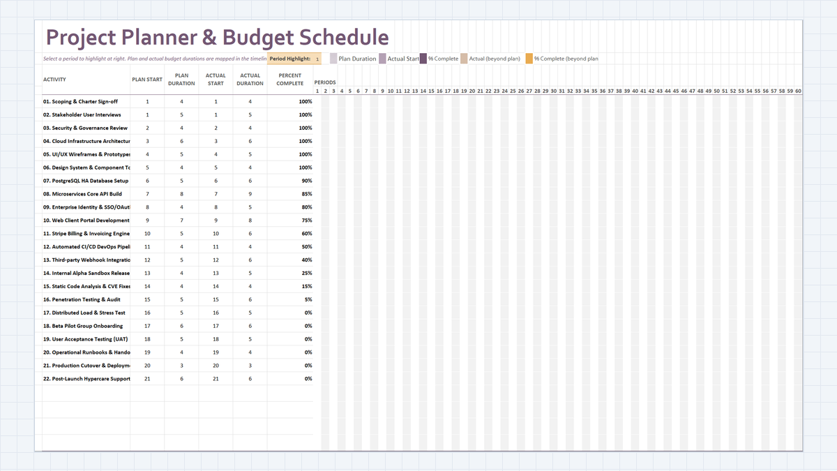
Build a Project Planner & Budget Schedule in Excel: 22 delivery workstreams, plan vs actual duration math, a dynamic in-cell Gantt chart, and percent-complete tracking that shows where schedule slippage starts.
 Project Management
Project Risk Register Excel Template
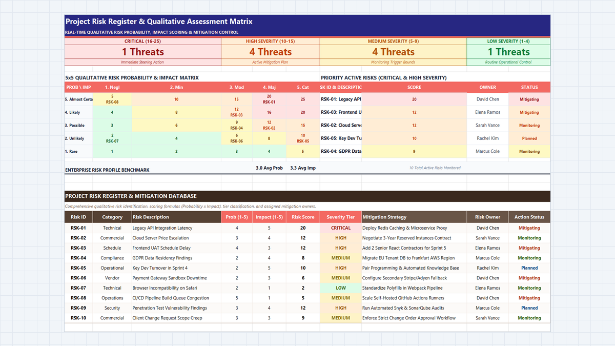
Learn enterprise risk governance in Microsoft Excel. Build an ISO 31000 and PMBOK-compliant 5x5 qualitative risk heatmap, automate probability and impact scoring, engineer multi-tier severity formulas, and enforce accountability with data validation.
Discussion
Ask questions, share formula tips, or discuss alternative approaches with fellow spreadsheet builders.
Loading discussion...