A founder tells you her company is worth "ten times earnings." An analyst calls a stock cheap because its P/E looks low. Both are using a shortcut, and both can be wrong. A business is worth the cash it will hand back to its owners in the future, not the profit printed on last year's income statement.
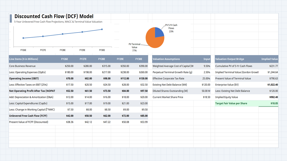
This DCF Valuation Model makes that idea concrete. On one sheet you project five years of free cash flow, discount each year back to today, add a terminal value for everything after year five, and end with a fair value per share. With a 9.50% WACC and 2.50% growth, this model lands at $18.05, against a market price of $18.50.
Why Earnings Multiples Are Not Enough
What Every DCF Template Needs
| Component | Where It Lives | What It Does |
|---|---|---|
| FCFF projection | B9:G17 | Turns revenue into unlevered free cash flow for FY26E to FY30E. |
| Discount rate (WACC) | J9, C18:G18 | 9.50% rate that converts each future cash flow into today's dollars. |
| Terminal value | J10, M10:M11 | Values everything after FY30E using 2.50% perpetual growth. |
| EV to equity bridge | M12:M15 | Subtracts $120.00 net debt and divides by 50.00 M shares. |
Build the Model Step by Step
1Step 1: Build the FCFF Engine and Format It
Type revenue, OpEx, D&A, CapEx, and working capital changes for FY26E to FY30E. Then build the rows in between: EBIT is revenue minus OpEx, taxes are EBIT times the tax rate, and NOPAT is EBIT minus taxes. Point the tax formula at $J$11 instead of typing 0.25, so changing the rate updates the whole model.
Free cash flow in row 17 is =C13+C14-C15-C16: NOPAT plus D&A, minus CapEx and working capital. It starts at $42.00 and grows to $85.00 by FY30E. Select C9:G18, press Ctrl + 1, choose Accounting with 2 decimals and the $ symbol, and the columns line up.
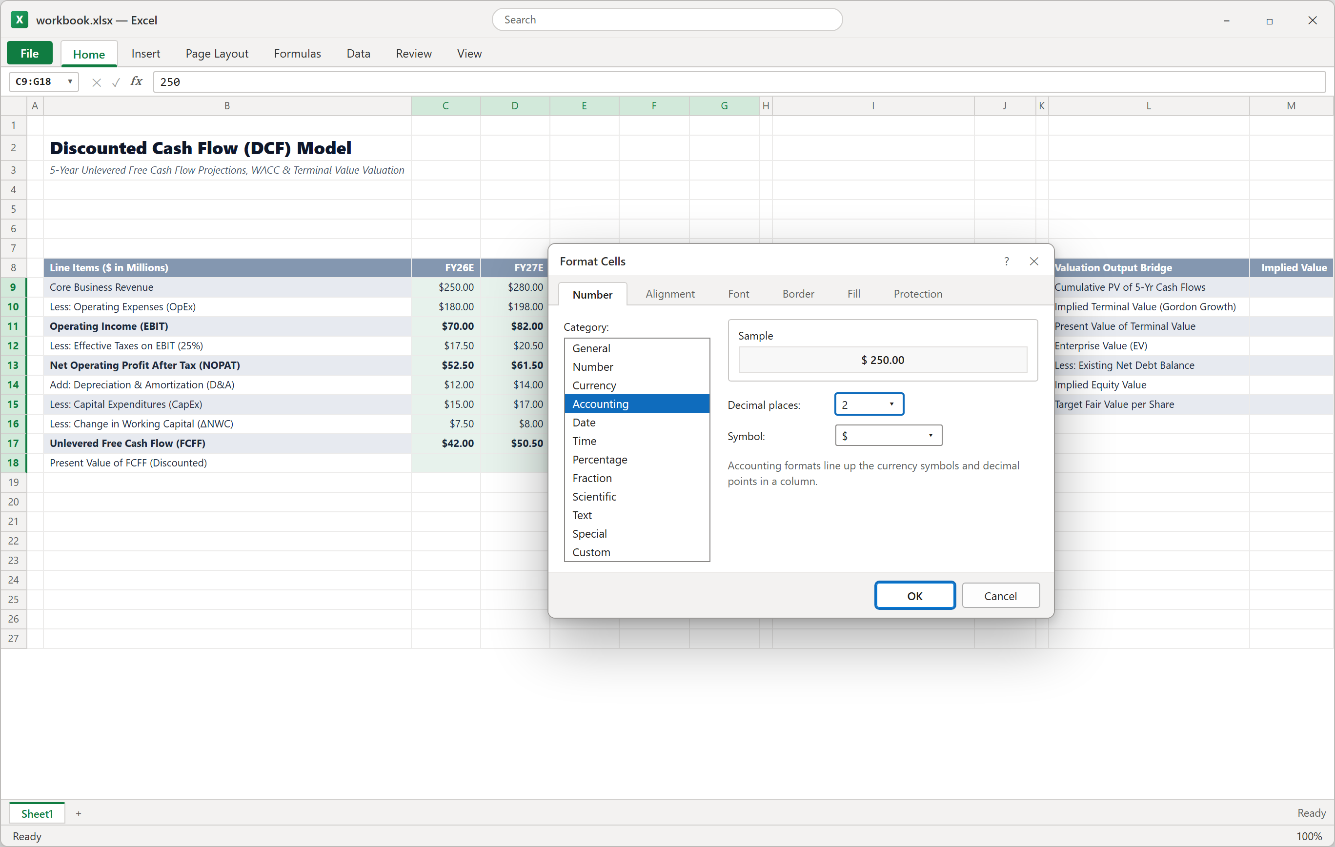
Figure 1: The FCFF rows in place, with Format Cells (Ctrl + 1) set to Accounting.
2Step 2: Discount Cash Flows with WACC
A dollar next year is worth less than a dollar today, so each year's cash flow gets divided by one plus the discount rate, raised to the year number. In C18, type =C17/(1+$J$9)^1.
While typing the reference to J9, press F4 to lock it as $J$9. Without the dollar signs, the reference slides when you copy across and you end up discounting with the wrong cell. Copy the formula to D18:G18 and change the exponent to 2, 3, 4, and 5. Press F2 on any cell to see its precedents color-coded.
FY26E becomes $38.36 and FY30E becomes $53.99. Add them in M9 with =SUM(C18:G18) to get $231.77.
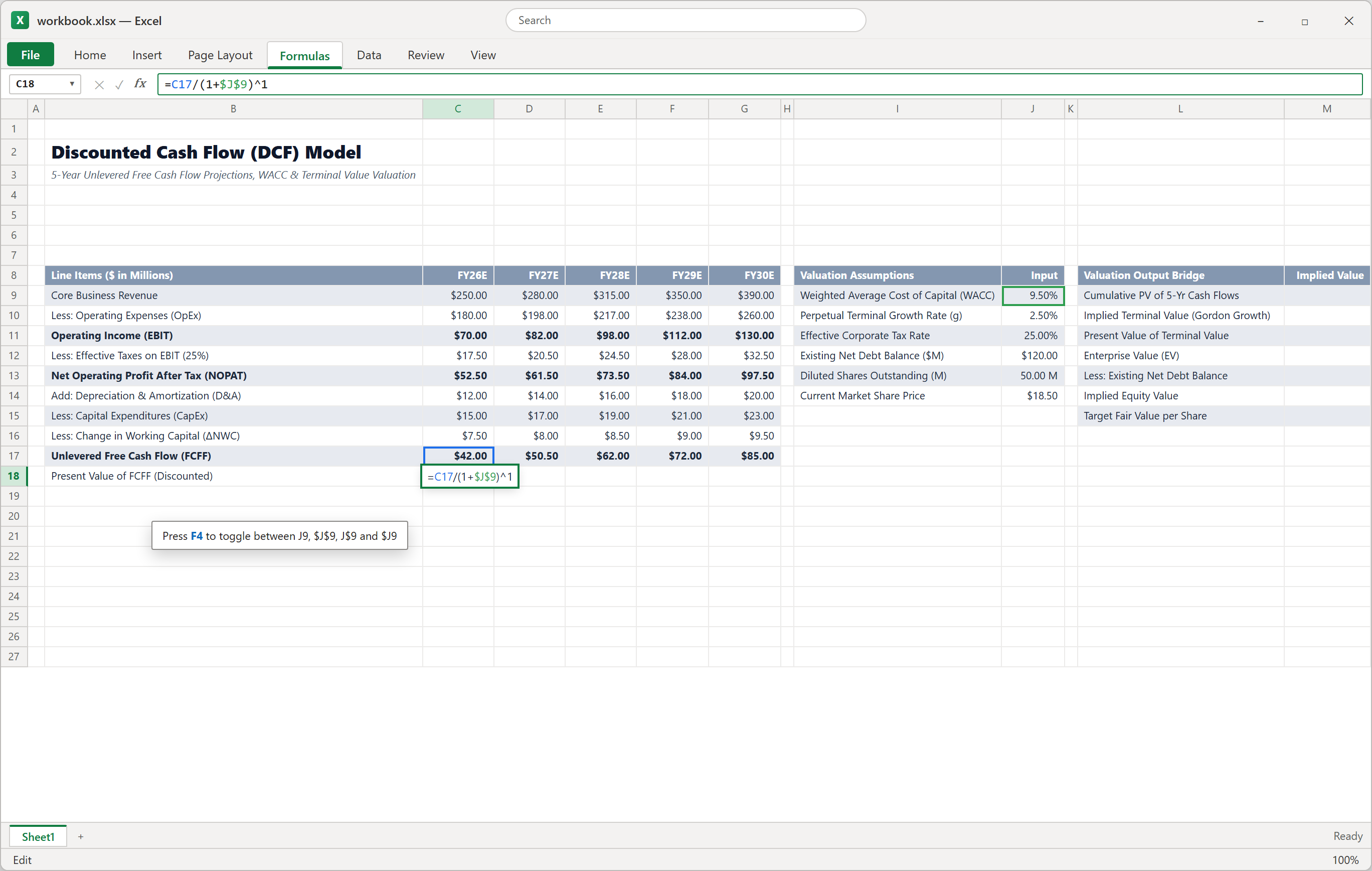
Figure 2: Discounting FY26E cash flow with the WACC cell locked.
3Step 3: Add Terminal Value and the Equity Bridge
The company does not stop in year five. In M10, use the Gordon Growth formula =(G17*(1+J10))/(J9-J10): final-year cash flow grown by 2.50%, divided by WACC minus growth. That gives $1,244.64. Discount it five years in M11 with =M10/(1+J9)^5 to get $790.63.
Enterprise value in M12 is M9 plus M11: $1,022.40. Subtract net debt in M13 and M14 to reach $902.40 of equity value. Divide that by shares in M15 to get $18.05 per share. Notice that terminal value is about 77% of enterprise value.
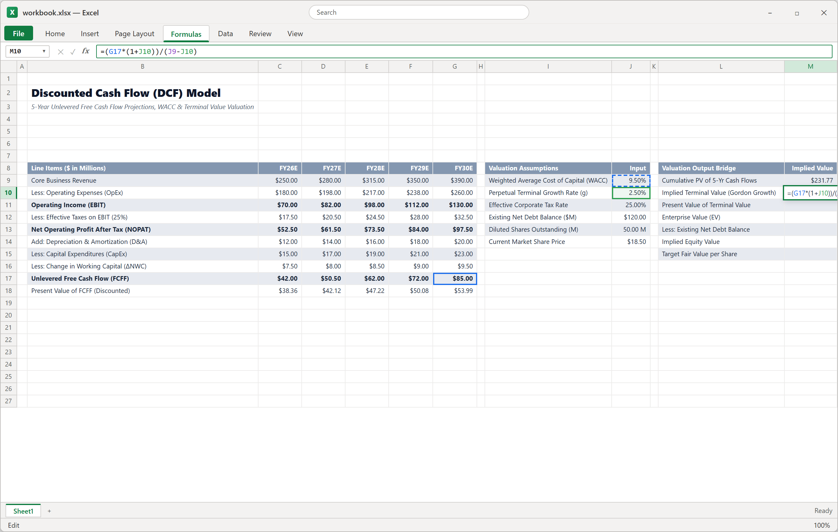
Figure 3: The Gordon Growth formula in M10 reads the last cash flow, g, and WACC.
4Step 4: Build a Two-Way Sensitivity Table
One answer hides a lot of uncertainty, so test a range. Below the model, in B22, type =M15. Put growth rates from 1.50% to 3.50% across C22:G22, and WACC from 8.50% to 10.50% down B23:B27.
Select B22:G27, open Data > What-If Analysis > Data Table, and set Row input cell to $J$10 and Column input cell to $J$9. Excel fills all 25 cells at once. The input cells must be on the same sheet as the table.
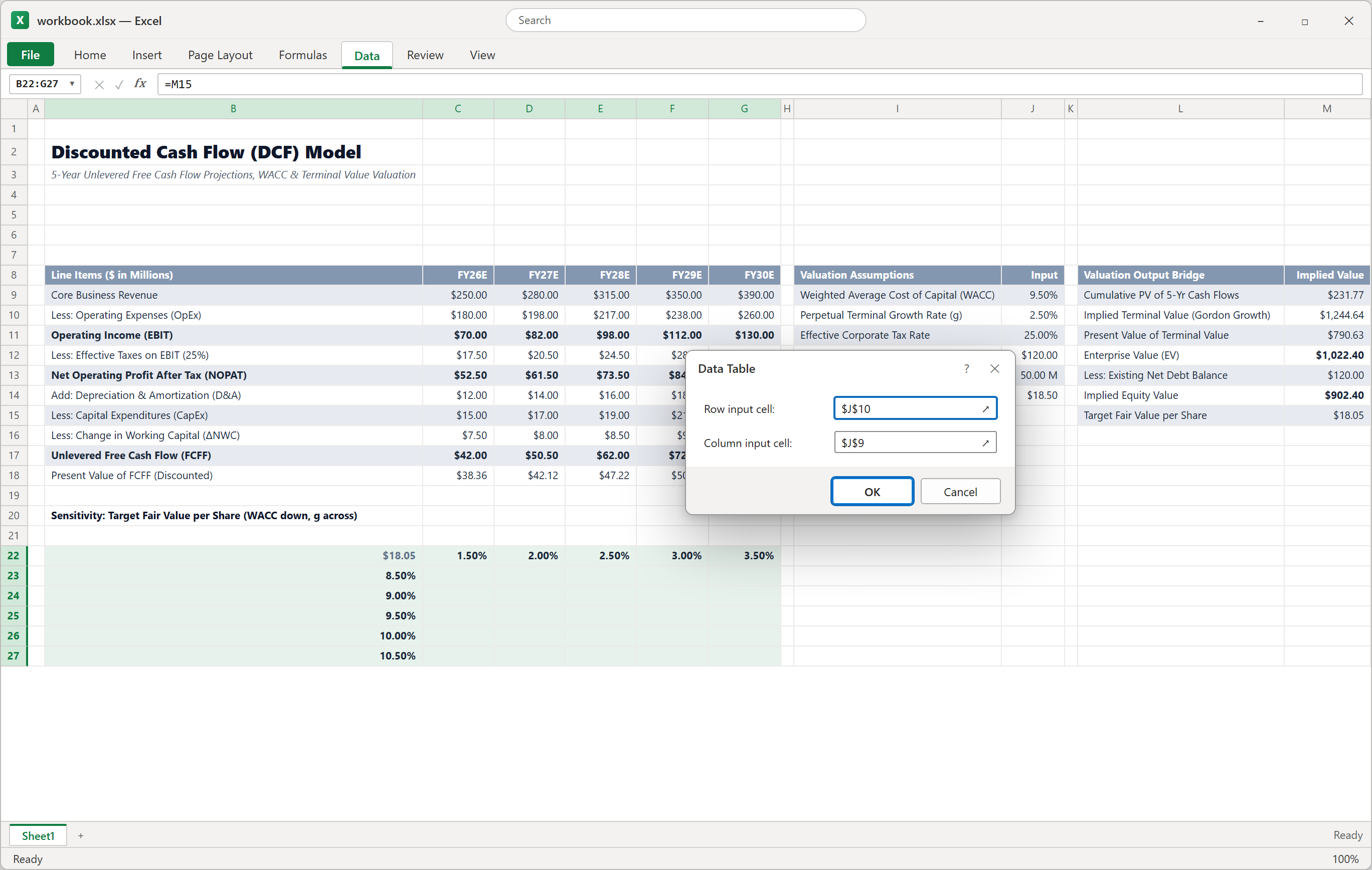
Figure 4: The Data Table dialog tells Excel which two inputs to vary.
5Step 5: Add a Conditional Formatting Alert
Make the answer announce itself. Select M15, open Home > Conditional Formatting > New Rule, and choose Format only cells that contain. Set Cell Value, less than, =$J$14, and pick a red fill.
Add a second rule for greater than or equal to =$J$14 with a green fill. Right now $18.05 sits below $18.50, so M15 turns red: the market price is about 2.5% above fair value, a hint that the shares look slightly expensive.
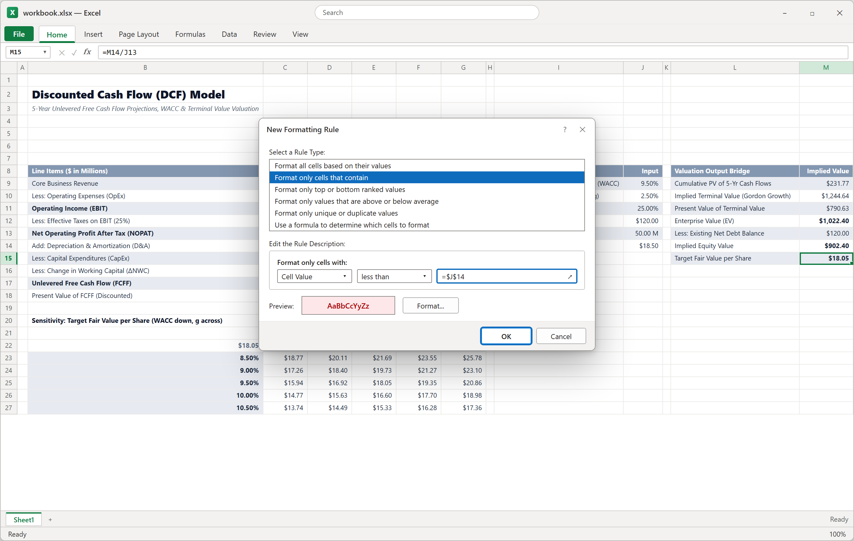
Figure 5: A rule that turns M15 red whenever fair value falls below the market price.
Sensitivity: Why Small WACC Changes Matter
| WACC | g 1.50% | g 2.00% | g 2.50% | g 3.00% | g 3.50% |
|---|---|---|---|---|---|
| 8.50% | $18.77 | $20.11 | $21.69 | $23.55 | $25.78 |
| 9.00% | $17.26 | $18.40 | $19.73 | $21.27 | $23.10 |
| 9.50% | $15.94 | $16.92 | $18.05 | $19.35 | $20.86 |
| 10.00% | $14.77 | $15.63 | $16.60 | $17.70 | $18.98 |
| 10.50% | $13.74 | $14.49 | $15.33 | $16.28 | $17.36 |
Data > What-If Analysis > Goal Seek, set M15 to 18.5 by changing J9. Excel returns a WACC of about 9.36%. Goal Seek overwrites J9, so type 9.50% back afterward.Download and Wrap-Up

Spreadsheet educator and web developer passionate about hands-on interactive spreadsheet practice.
Related Practical Exercises
Explore more hands-on spreadsheet models with downloadable practice workbooks.
 Finance
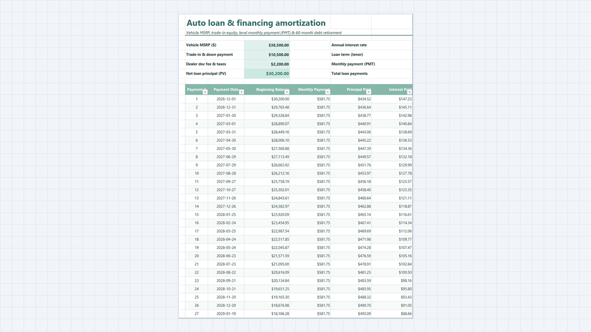
Auto Loan Calculator Excel Template
Know your exact monthly car payment and total loan interest before you visit the dealership. Learn how this auto loan calculator works, explore its workbook structure, and follow a clear step-by-step guide to build it in Excel with PMT and amortization formulas.
 Productivity
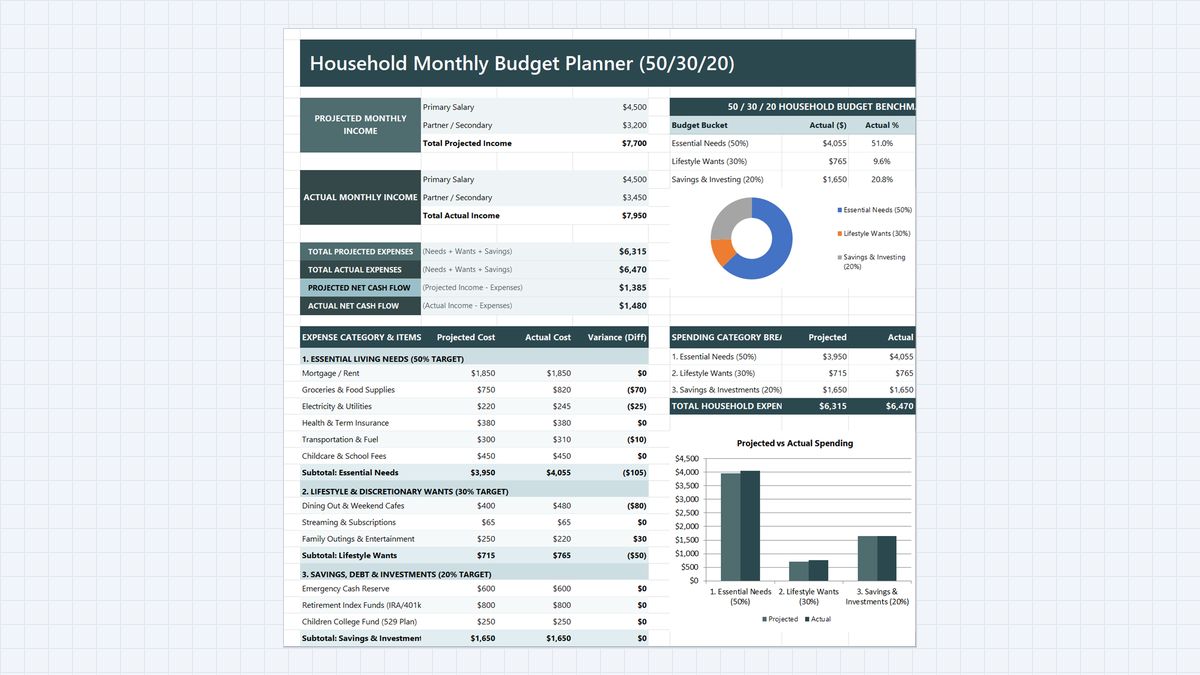
Household Budget Planner Excel Template
Find out where a two-income family's money really goes. Build a household budget planner in Microsoft Excel with 50/30/20 buckets, projected vs actual variance, a net cash flow card, and automatic over-budget alerts.
 Project Management
Project Timeline Tracker Excel Template
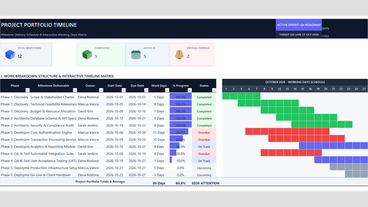
Keep sprint deadlines and client milestones on track without messy calendar math. Build a Project Timeline Tracker Excel Template with automatic working days using NETWORKDAYS, single-owner dropdowns, progress bars, and portfolio health alerts.
 Finance
Loan Payoff Calculator Excel Template
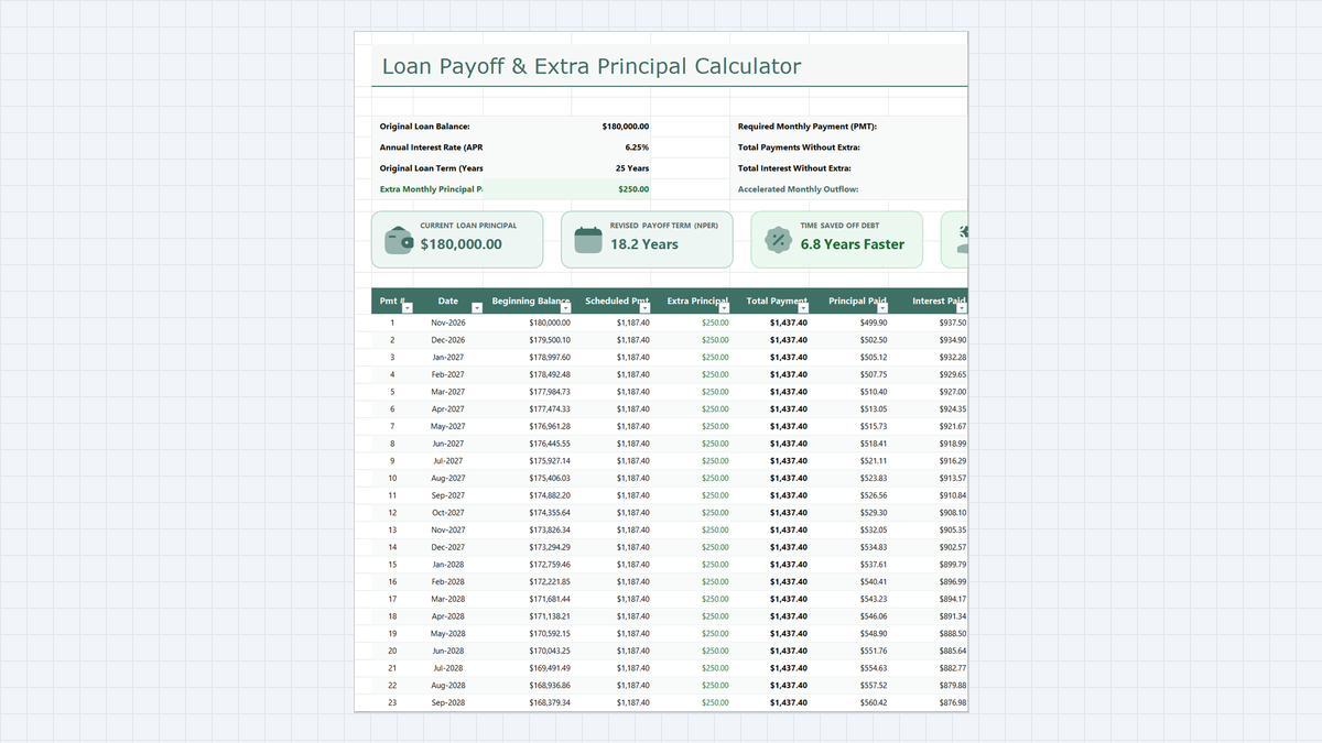
See how extra principal payments shorten a loan. Build a loan payoff calculator in Microsoft Excel with a PMT-based payment, a monthly amortization schedule, and the interest-versus-principal split behind every payment.
 Finance
Leveraged Buyout (LBO) Model Excel Template
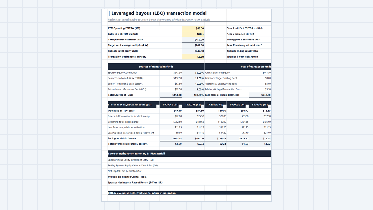
Build a 5-year leveraged buyout (LBO) model in Microsoft Excel. Set entry valuation, balance a sources and uses table, run a debt paydown schedule with an 80% cash sweep, and calculate sponsor MoIC and IRR.
Discussion
Ask questions, share formula tips, or discuss alternative approaches with fellow spreadsheet builders.
Loading discussion...