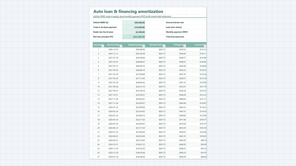
Walking into a car dealership without your own numbers puts you at an immediate disadvantage. The most common question a car salesperson will ask you is simple: "What monthly payment are you looking for?" While that sounds helpful, it is actually a classic sales tactic. When you focus only on the monthly installment, the finance manager can easily stretch your loan from 48 months to 72 or 84 months. Your monthly bill drops slightly, but your total interest charges can double or triple over the life of the loan.
To make matters worse, dealerships often bundle document fees, sales taxes, and vehicle trade-in credits into confusing paperwork. Without a clear spreadsheet in front of you, it is hard to tell how much you are truly borrowing. This Auto Loan Calculator Excel Template gives you total clarity. By calculating your exact numbers beforehand, you can walk into the showroom with confidence, knowing every single dollar that goes toward the car, the bank, and dealer fees.
The Real-World Car Dealership Problem
Why This Template Protects Your Wallet
PMT function with proper monthly interest rate division, the template matches the exact penny figures used by commercial banks, credit unions, and auto lenders.Workbook Layout and Cell Structure
| Cell Range | Parameter Name | Data Type | Number Format | Description and Formula Rule |
|---|---|---|---|---|
| D4 | Vehicle MSRP / Price | User Input | Accounting ($#,##0.00) | Agreed purchase price of the vehicle ($38,500.00). |
| D5 | Trade-in and Down Payment | User Input | Accounting ($#,##0.00) | Total upfront equity: $6,500 trade-in credit plus $4,000 cash down payment ($10,500.00). |
| D6 | Dealer Doc Fee and Taxes | User Input | Accounting ($#,##0.00) | Estimated documentation fees, registration, and state sales taxes ($2,200.00). |
| D7 | Net Loan Principal (PV) | Formula Output | Accounting ($#,##0.00) | =D4-D5+D6. True starting loan balance ($30,200.00) financed through the bank. |
| H4 | Annual Interest Rate (APR) | User Input | Percentage (0.00%) | Annual percentage rate quoted by lender (5.85%). Divided by 12 in monthly calculations. |
| H5 | Loan Term (Tenor) | User Input | Custom (0 "Months") | Total duration of the loan in months (60 months = 5 years). |
| H6 | Monthly Payment (PMT) | Formula Output | Accounting ($#,##0.00) | =ROUND(PMT(H4/12, H5, -D7), 2). Fixed monthly payment required ($581.65). |
| H7 | Total Loan Payments | Formula Output | Accounting ($#,##0.00) | =ROUND(H6*H5, 2). Total cash paid to the lender across all 60 months ($34,899.00). |
| B10:H69 | Amortization Ledger | Monthly Schedule | Accounting ($#,##0.00) | 60 payment rows showing Beginning Balance, Monthly Payment, Principal Paid, Interest Paid, and Ending Balance. |
| B70:H70 | Total Rollup Row | Formula Summary | Accounting ($#,##0.00) | Final totals using =SUM(E10:E69), =SUM(F10:F69), and =SUM(G10:G69) confirming a zero ending balance. |
With this blueprint clear, let us walk through the exact steps to build this template in Microsoft Excel, following the real screenshots from the workbook.
Step-by-Step Build Guide with Real Screenshots
1Step 1: Calculate Net Loan Principal (D4 - D5 + D6)
Before calculating any interest or payments, you must know the exact dollar amount being financed through your bank or credit union. Many people make the mistake of using the car sticker price as the loan balance, but that ignores upfront credits and extra fees.
In cell D4, enter the agreed vehicle purchase price ($38,500.00). In cell D5, enter the total upfront credit, which includes both your old car trade-in allowance and your cash down payment ($10,500.00). In cell D6, enter dealer documentation fees and local registration taxes ($2,200.00).
Now, select cell D7 and type the formula: =D4-D5+D6. This takes the car price, subtracts your upfront equity, and adds the fees back in. The result is $30,200.00. This is your net capitalized cost, and it represents the true principal value (PV) for your loan.
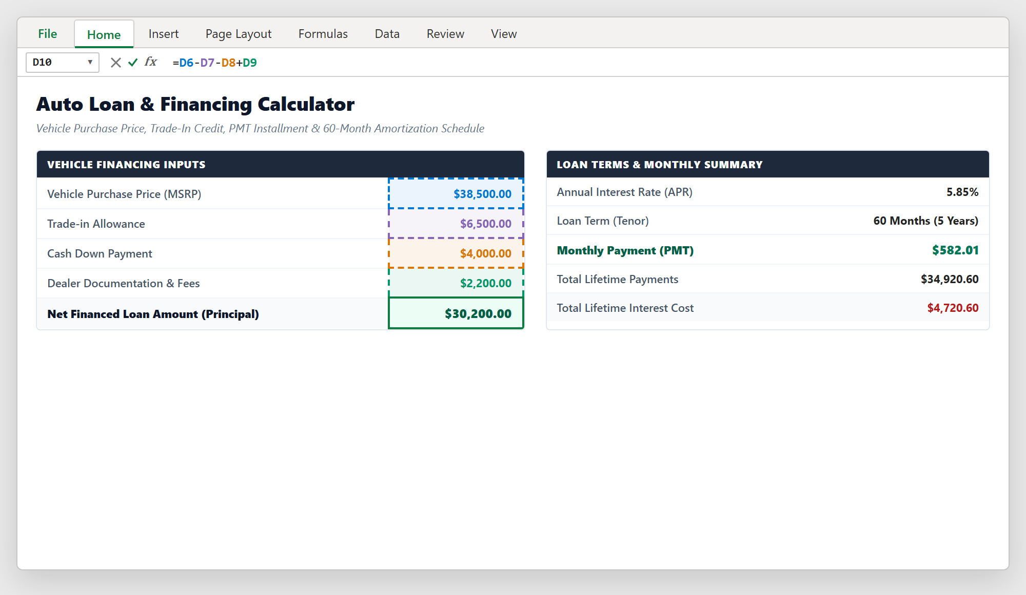
Figure 1: Calculating net capitalized loan principal in cell D7 by combining vehicle purchase price with dealer fees and subtracting upfront trade-in equity.
2Step 2: Calculate Fixed Monthly Payment with PMT
Once your loan principal is set in cell D7, you can calculate the exact level monthly installment using Excel's financial PMT function.
The PMT function requires three main arguments: =PMT(rate, nper, pv). In auto loans, interest rates are quoted on an annual basis (APR), but payments occur monthly. Therefore, you must divide the annual rate by 12: H4/12 (5.85% / 12 = 0.4875% per month). The second argument is the total number of monthly payments: H5 (60 months).
The third argument is the present value (principal). In Excel, financial formulas follow cash flow signs: money you borrow is an inflow, and payments you make are outflows. To make your monthly payment display as a clean positive dollar amount, place a minus sign in front of the principal cell: -D7. Finally, wrap the calculation in ROUND(..., 2) to prevent fractional penny drift.
Select cell H6 and type: =ROUND(PMT(H4/12, H5, -D7), 2). Press Enter. Your fixed monthly payment will immediately display as $581.65.
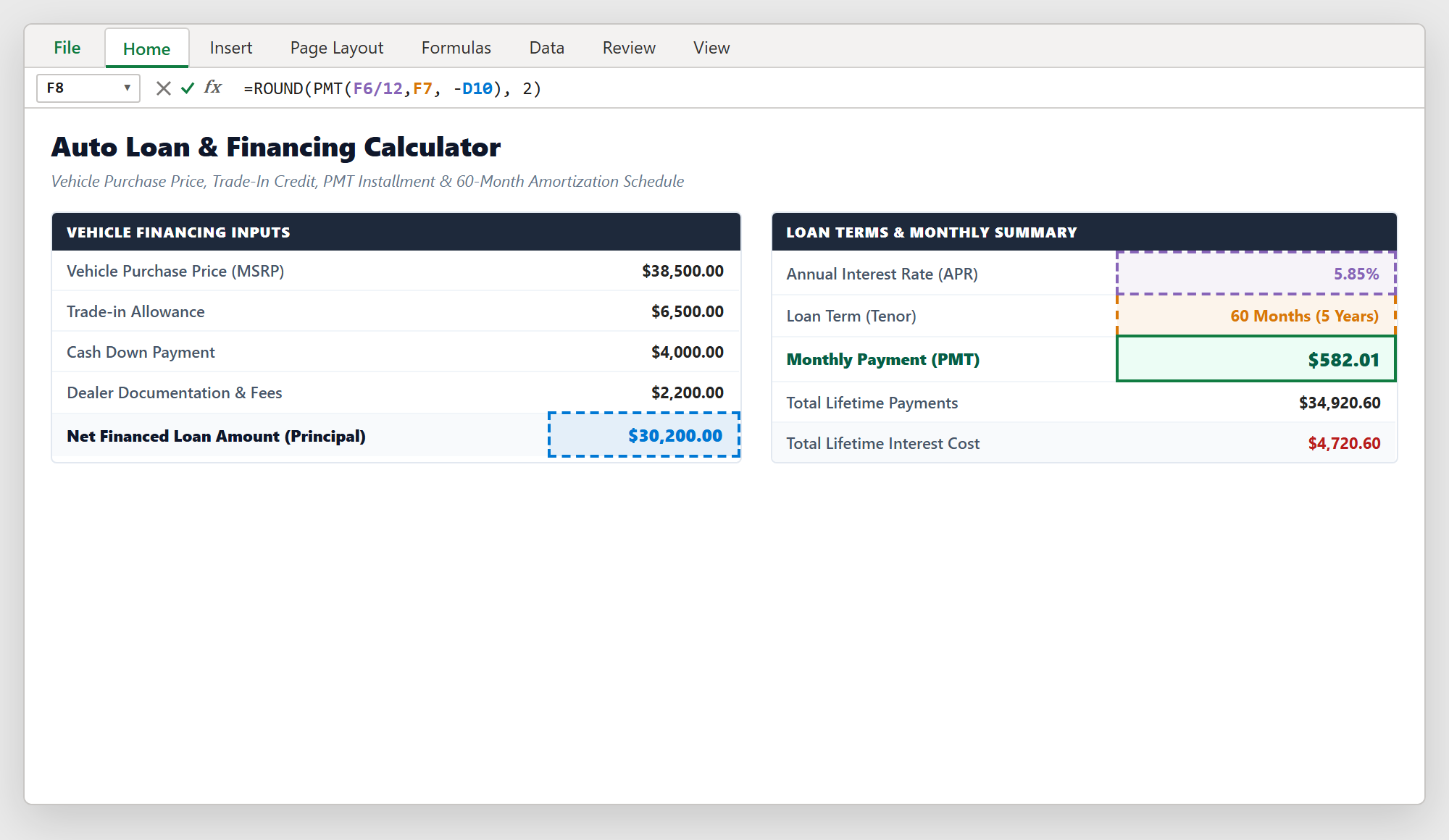
Figure 2: Calculating level monthly payment in cell H6 using PMT with monthly rate conversion and cash outflow sign rules.
3Step 3: Format Financial Cells with Accounting Format
Raw numbers like 581.65 or 30200 look messy and hard to read on a financial summary. To give your spreadsheet a professional appearance, apply standard Accounting formatting.
Highlight your input cells (D4:D7 and H6:H7) as well as the schedule columns below. Press Ctrl + 1 on Windows (or Cmd + 1 on Mac) to open the Format Cells window.
Click on the Accounting category on the left. Set Decimal places to 2, and pick the $ symbol from the currency dropdown. Click OK. This cleanly aligns all decimal points in a straight vertical line, places the dollar sign flush against the left cell border, and formats any future zero balances as neat hyphens.
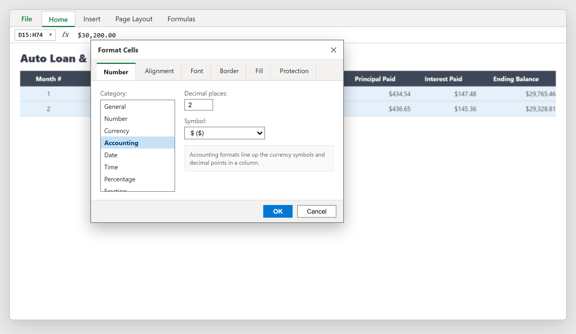
Figure 3: Setting the Accounting number format via Format Cells (Ctrl + 1) for clean dollar signs and vertical decimal alignment.
4Step 4: Separate Monthly Interest and Principal
Each month, your fixed payment of $581.65 is divided into two parts: interest paid to the lender and principal paid toward owning the car.
In Month 1 (Row 10), your starting loan balance in cell D10 links directly to your net loan principal: =D7 ($30,200.00). Your scheduled payment in cell E10 links to your fixed payment: =$H$6. Notice the dollar signs locking cell H6 so it stays fixed when copied down.
Next, calculate the interest charge for that first month in cell G10: =ROUND(D10*($H$4/12), 2). This multiplies your beginning balance by the monthly interest rate, yielding $147.23 in interest expense.
Now, subtract that interest from your total payment to find how much principal you paid in cell F10: =E10-G10 ($581.65 - $147.23 = $434.42). Finally, calculate your ending balance in cell H10: =D10-F10 ($30,200.00 - $434.42 = $29,765.58).
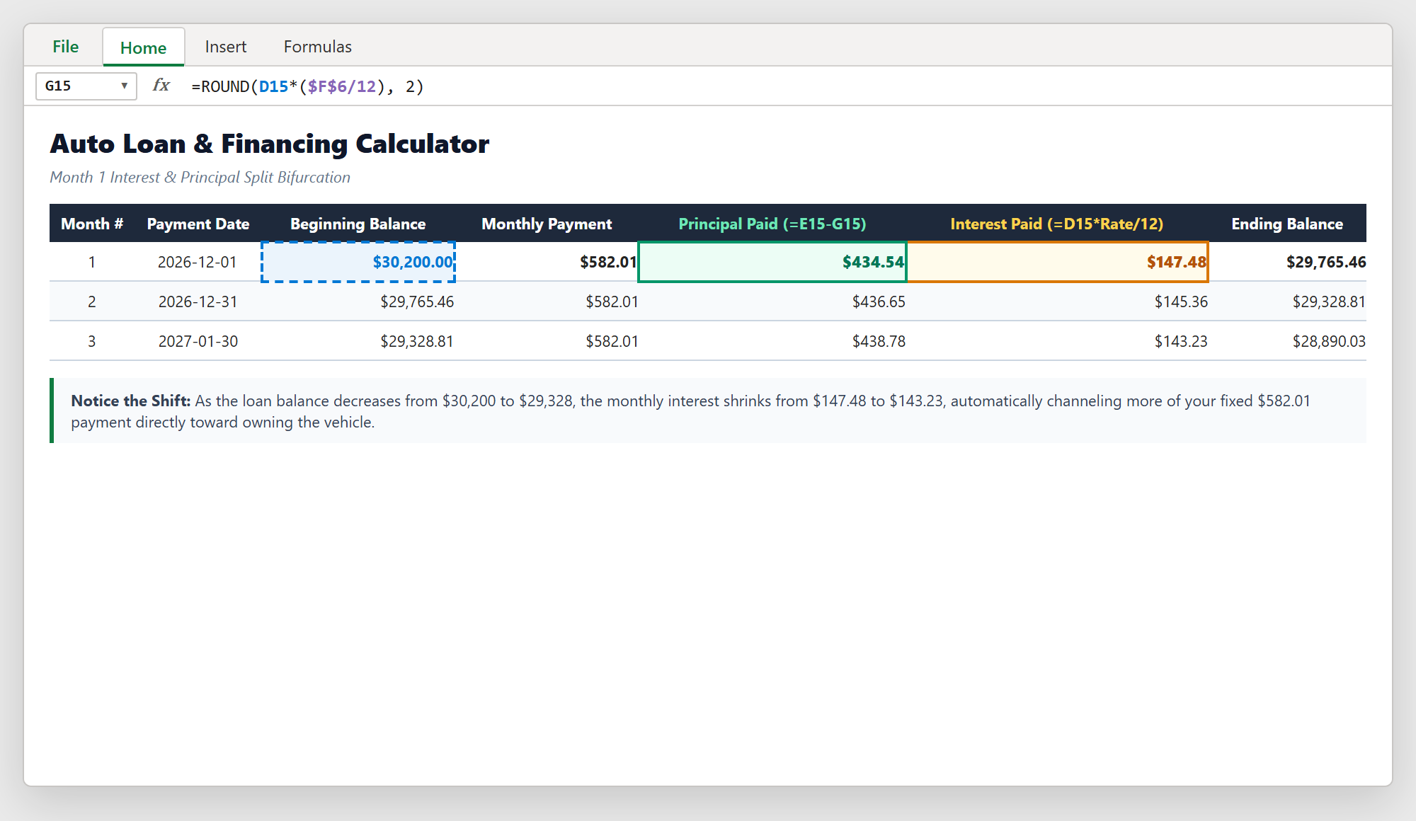
Figure 4: Splitting the monthly payment in Row 10 into monthly interest charges and direct principal reduction.
5Step 5: Build the 60-Month Amortization Schedule
Now that Month 1 is complete, you can build an unbroken chain across all 60 months.
For Month 2 (Row 11), the new beginning balance must equal the previous month's ending balance. In cell D11, type: =H10. Never retype or hardcode this number manually. By linking to cell H10, any prepayment or rate change will smoothly update through the entire schedule.
Copy the formulas in cells E10:H10 down across rows 11 to 69. As you scroll down, you will notice a satisfying pattern: each month, as your loan balance drops, the interest charge shrinks. Because your total payment stays constant at $581.65, more of your money goes toward principal every single month.
In Row 70, create a summary total row. Use =SUM(E10:E69) for total payments ($34,899.00), =SUM(F10:F69) for total principal paid ($30,200.00), and =SUM(G10:G69) for total interest charges ($4,699.00). Look at cell H69 at Month 60: your ending loan balance reaches exactly $0.00, proving that your loan is fully paid off.
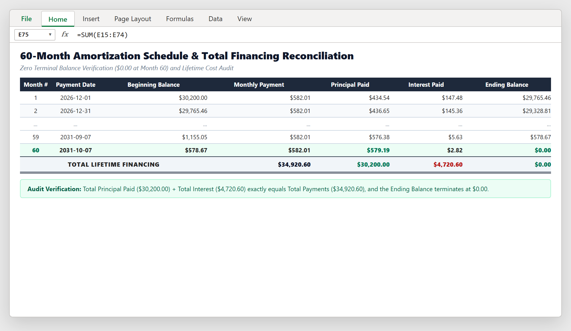
Figure 5: Complete 60-month amortization schedule confirming that total principal paid matches original borrowing and ends at zero balance.
Comparing Loan Terms: 48, 60, and 72 Months
Monthly Payment: $707.82 | Total Interest Paid: $3,775.36 | Total Cost: $33,975.36.
Analysis: Your monthly payment is higher, but you pay off the car a full year earlier and save nearly $1,000 in interest compared to a 5-year loan.
Monthly Payment: $581.65 | Total Interest Paid: $4,699.00 | Total Cost: $34,899.00.
Analysis: This is the most common auto loan duration. It strikes a manageable balance between a reasonable monthly payment and a moderate total interest charge.
Monthly Payment: $498.05 | Total Interest Paid: $5,659.60 | Total Cost: $35,859.60.
Analysis: While saving $83 per month might seem attractive, you end up paying an extra $960 in pure interest to the lender. Even worse, long loans keep you "underwater" (owing more than the car is worth) for much longer as the vehicle depreciates.
Common Formula Mistakes and Dealership Traps
=PMT(H4, H5, -D7) without dividing cell H4 by 12, Excel assumes you are paying 5.85% interest every single month. Your monthly payment will show up as thousands of dollars. Always write H4/12 in the rate argument.=PMT(H4/12, H5, D7) without a minus sign, Excel will return -$581.65 in red text or parentheses. In financial math, cash you pay out is an outflow, so reversing the sign makes your monthly payment display as a clean positive value.Conclusion and Download Your Free Template

Spreadsheet educator and web developer passionate about hands-on interactive spreadsheet practice.
Related Practical Exercises
Explore more hands-on spreadsheet models with downloadable practice workbooks.
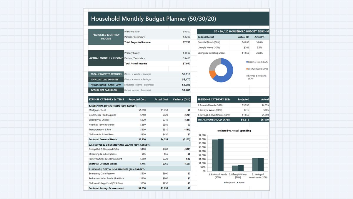 Productivity
Household Budget Planner Excel Template
Find out where a two-income family's money really goes. Build a household budget planner in Microsoft Excel with 50/30/20 buckets, projected vs actual variance, a net cash flow card, and automatic over-budget alerts.
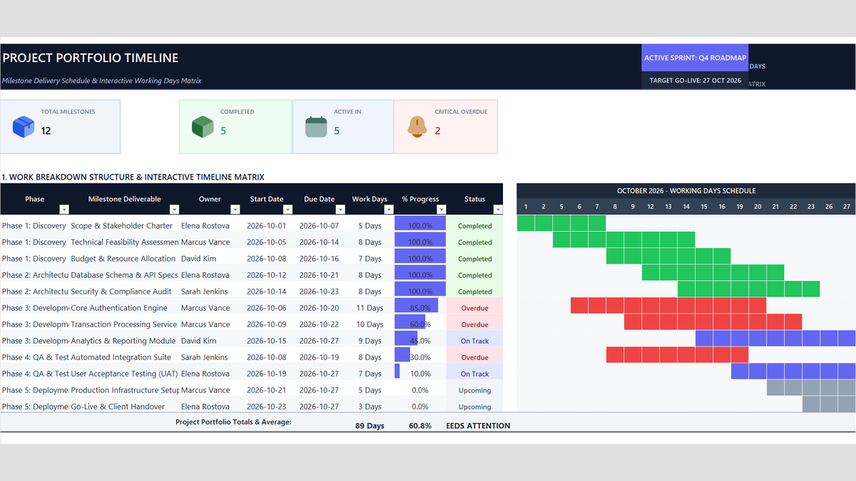 Project Management
Project Timeline Tracker Excel Template
Keep sprint deadlines and client milestones on track without messy calendar math. Build a Project Timeline Tracker Excel Template with automatic working days using NETWORKDAYS, single-owner dropdowns, progress bars, and portfolio health alerts.
 Finance
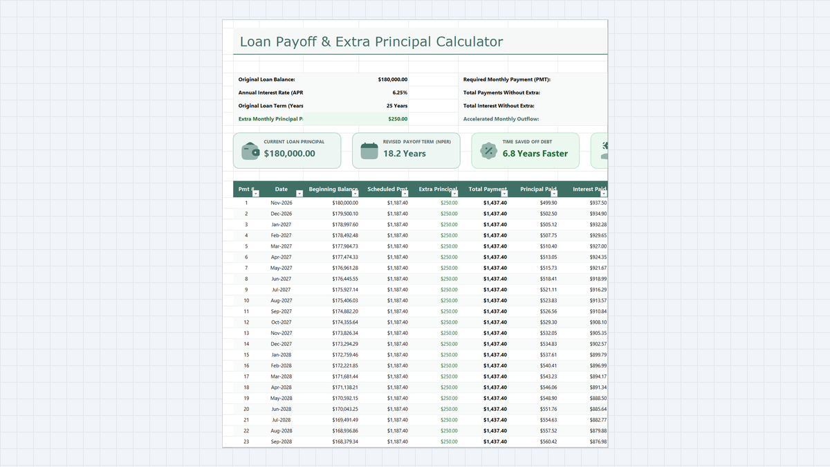
Loan Payoff Calculator Excel Template
See how extra principal payments shorten a loan. Build a loan payoff calculator in Microsoft Excel with a PMT-based payment, a monthly amortization schedule, and the interest-versus-principal split behind every payment.
 Finance
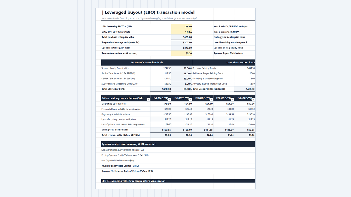
Leveraged Buyout (LBO) Model Excel Template
Build a 5-year leveraged buyout (LBO) model in Microsoft Excel. Set entry valuation, balance a sources and uses table, run a debt paydown schedule with an 80% cash sweep, and calculate sponsor MoIC and IRR.
 Sales
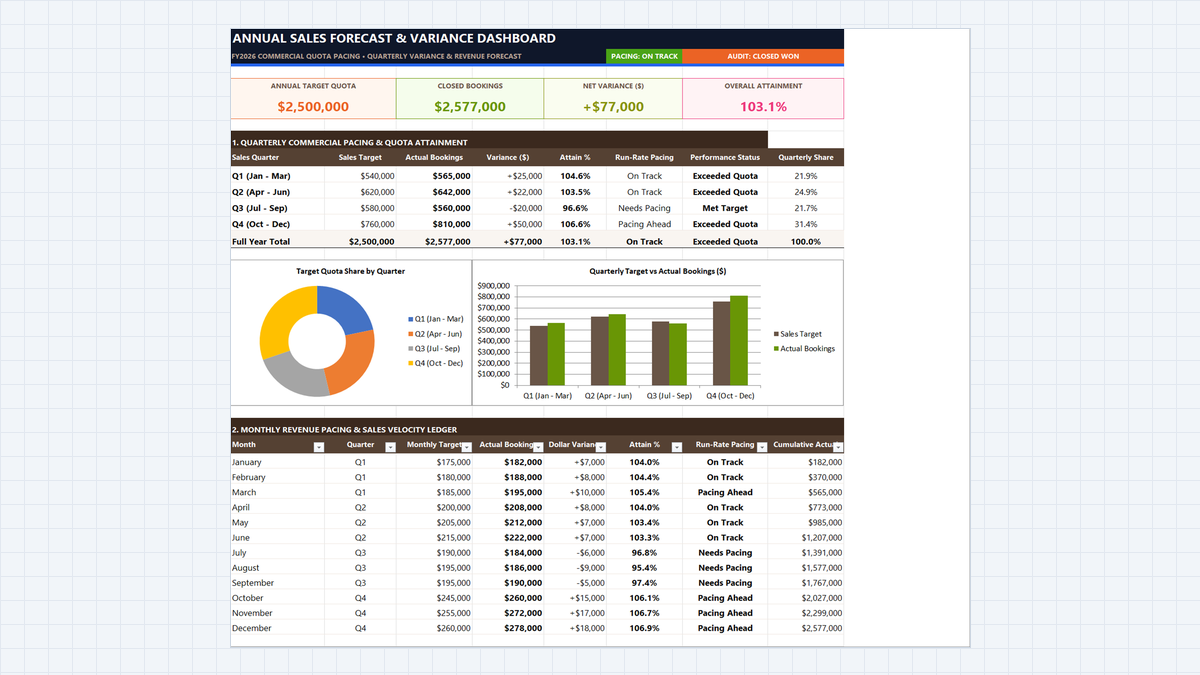
Sales Forecast Template Excel (Annual Model)
Learn commercial revenue forecasting in Microsoft Excel. Build an annual sales forecasting dashboard featuring quarterly variance calculations, dynamic quota attainment metrics, clustered column comparison charts, and executive pacing scorecards.
Discussion
Ask questions, share formula tips, or discuss alternative approaches with fellow spreadsheet builders.
Loading discussion...