Why Every Cash Register Needs a Daily Ledger
If you run a retail shop, coffee bar, or small office, physical cash changes hands dozens of times a day. A customer pays with cash, an employee buys printer paper, or a repair technician asks for immediate payment from the cash box. Without a simple daily record, finding out why $50 is missing at the end of the week takes hours of painful receipt hunting.
A daily cash book solves this problem completely. It acts as a clear financial journal where every dollar coming in (debit) and every dollar going out (credit) is written down the moment it happens. By keeping a live running balance, you can compare the number on your screen to the physical bills in your cash drawer in thirty seconds flat.
In this exercise, you will build a clean, practical cash ledger in Excel. You will learn how to prevent typos with category dropdowns, calculate running balances automatically, highlight accidental negative balances in bright red, and summarize your monthly expenses so tax preparation takes minutes.
Table Columns & Data Dictionary
Our cash workbook is organized into a clean single-sheet layout. The primary transaction ledger spans columns B through I (rows 16 to 27), while the top right corner holds our monthly category expense summary (columns J and K). Below is the exact data layout used in the downloadable template.
| Column | Field Name | Data Type | Number Format | Description & Modeling Rule |
|---|---|---|---|---|
| B | No. | Integer Sequence | Center Align | Sequential line number for each cash transaction (1, 2, 3...). |
| C | Date | Calendar Date | YYYY-MM-DD | The exact day the cash moved into or out of the register. |
| D | Voucher # | Text Code | Center Align | Receipt or petty cash voucher number (e.g. OB-2026, JV-001) for physical audit receipts. |
| E | Account Category | Dropdown List | Text | Standardized expense or revenue category locked via Data Validation. |
| F | Transaction Description | Text | Left Align | Plain English memo explaining who received the money or where the cash came from. |
| G | Debit Inflow ($) | Numeric Currency | $#,##0.00 | Cash received into the register (cash sales, client deposits, cash injections). |
| H | Credit Outflow ($) | Numeric Currency | $#,##0.00 | Cash paid out of the register (supplies, courier fees, sanitation services). |
| I | Running Balance ($) | Formula Calculation | $#,##0.00 (Bold) | =Prior Balance + Debit Inflow - Credit Outflow. Shows available cash on hand. |
Building Your Daily Cash Book Step by Step
Follow these four simple steps to build your operational cash ledger. We will start with input safeguards, connect our live running math, set up an automatic alert, and finish with a monthly expense breakdown.
3.1Step 1: Adding Category Dropdowns with Data Validation
When different team members write down cash transactions, one person might type "Cleaning", another writes "Janitorial", and a third writes "Facilities". Later, when you want to see how much you spent on office upkeep, your formulas cannot group them together because the names do not match.
We fix this in two clicks by restricting the Account Category column to an approved list of options.
Select cells D17 through D27 in your table. On the top ribbon, click the Data tab, then click the Data Validation button.
In the dialog box, under Allow, choose List. In the Source box, type your standard categories separated by commas: "Sales Receipts, Facilities, Shipping, Travel, Consumables, Repairs". Make sure In-cell dropdown is checked and click OK.
Now, whenever someone logs an entry, a small arrow appears allowing them to pick the right category instantly without spelling mistakes.
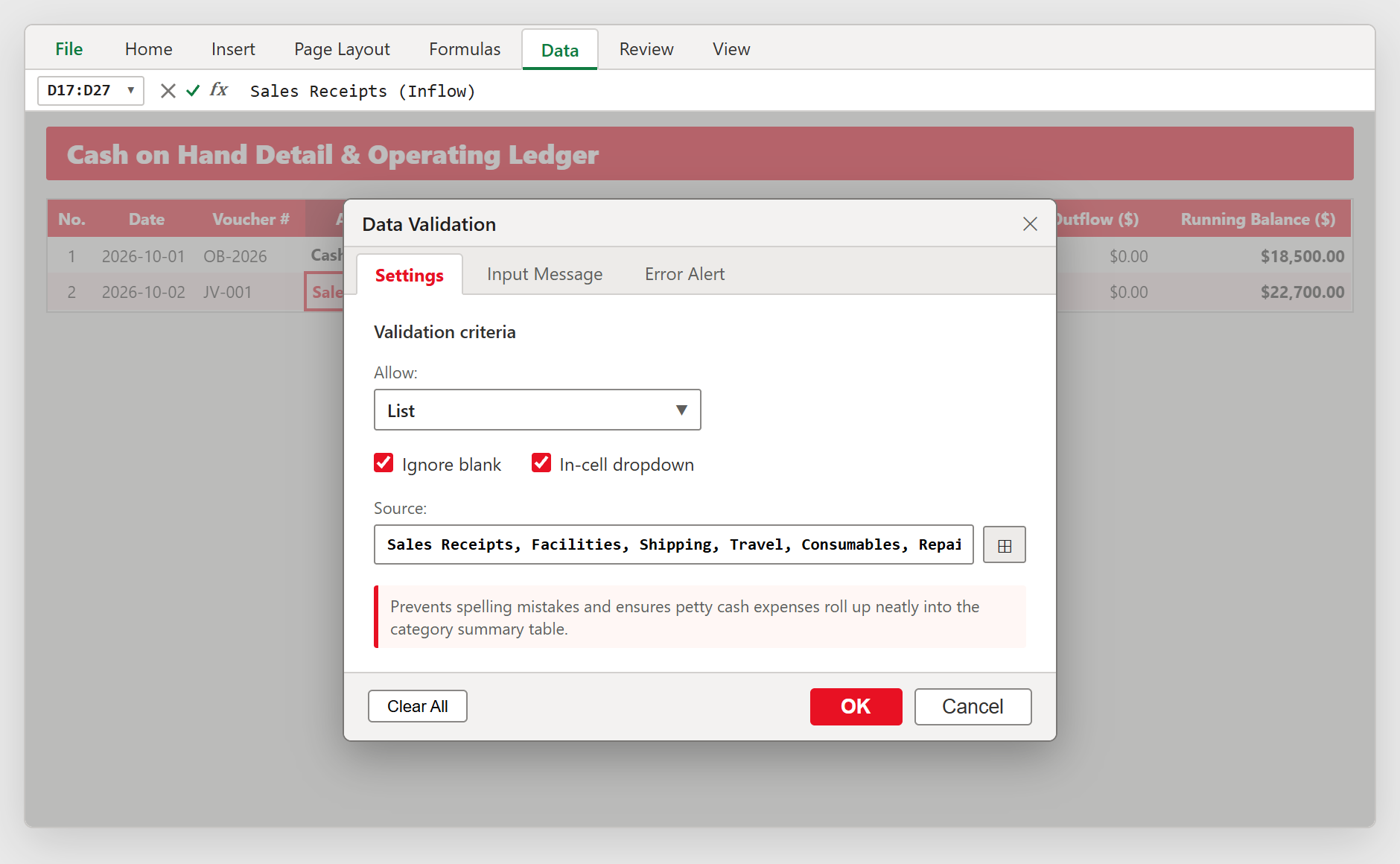
Figure 1: Locking the Account Category column to a standard dropdown list using Excel Data Validation.
3.2Step 2: Calculating Live Running Cash Balances
Your cash ledger needs to show the exact dollar amount sitting in your cash drawer at any moment. To do this, we use a simple arithmetic formula that carries over the previous balance, adds today cash in, and subtracts today cash out.
Row 17 contains our opening balance forward: $18,500.00 in cell H17.
In Row 18, we receive $4,200.00 from customer sales (cell F18) with $0.00 paid out (cell G18). To find our new balance, click on cell H18 and type: =H17+F18-G18.
Press Enter. Excel calculates $22,700.00. Now grab the small green fill handle in the lower right corner of cell H18 and drag it down to Row 27. Every row now recalculates instantly as new receipts and expenses are recorded.
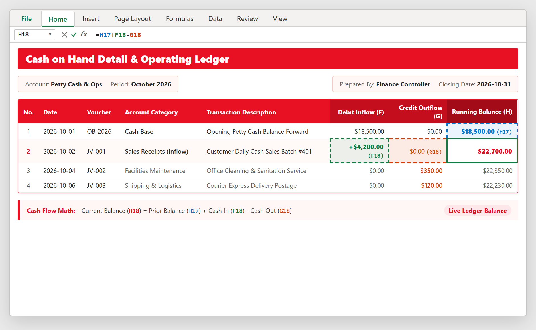
Figure 2: Formulating the live running cash balance in cell H18 (=H17+F18-G18) with color-coded cell highlights.
3.3Step 3: Setting Up Red Alerts for Negative Cash
Physical cash cannot drop below zero. You cannot hand a customer minus ten dollars. If your cash book shows a negative balance, it means an expense was logged under the wrong date or a cash sale was forgotten.
We can ask Excel to immediately warn us with a soft red fill if the balance ever dips into the negative.
Highlight your running balance column (cells H17:H27). On the Home tab, click Conditional Formatting, then click New Rule.
Select "Format only cells that contain". In the rule description, choose "Cell Value", change the dropdown to "less than", and type 0 in the box. Click Format, pick a light red fill with dark red text, and click OK.
If someone accidentally enters an outflow larger than available cash, the cell instantly glows red, prompting the manager to review the register drawer before closing.
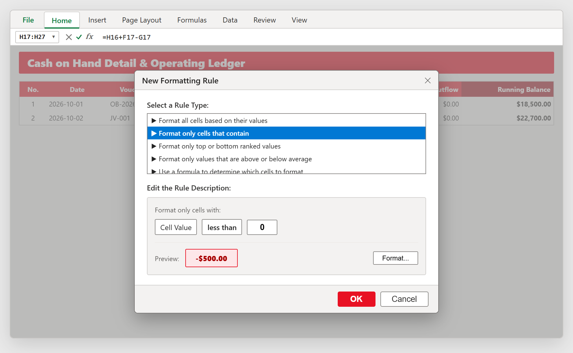
Figure 3: Creating an automatic negative overdraft alert rule in Excel Conditional Formatting to catch accounting mistakes early.
3.4Step 4: Grouping Expenses by Category with SUMIF
At the end of the month, business owners do not want to scroll through hundreds of individual receipts. They want to know the big picture: how much did we spend on shipping, repairs, and office supplies?
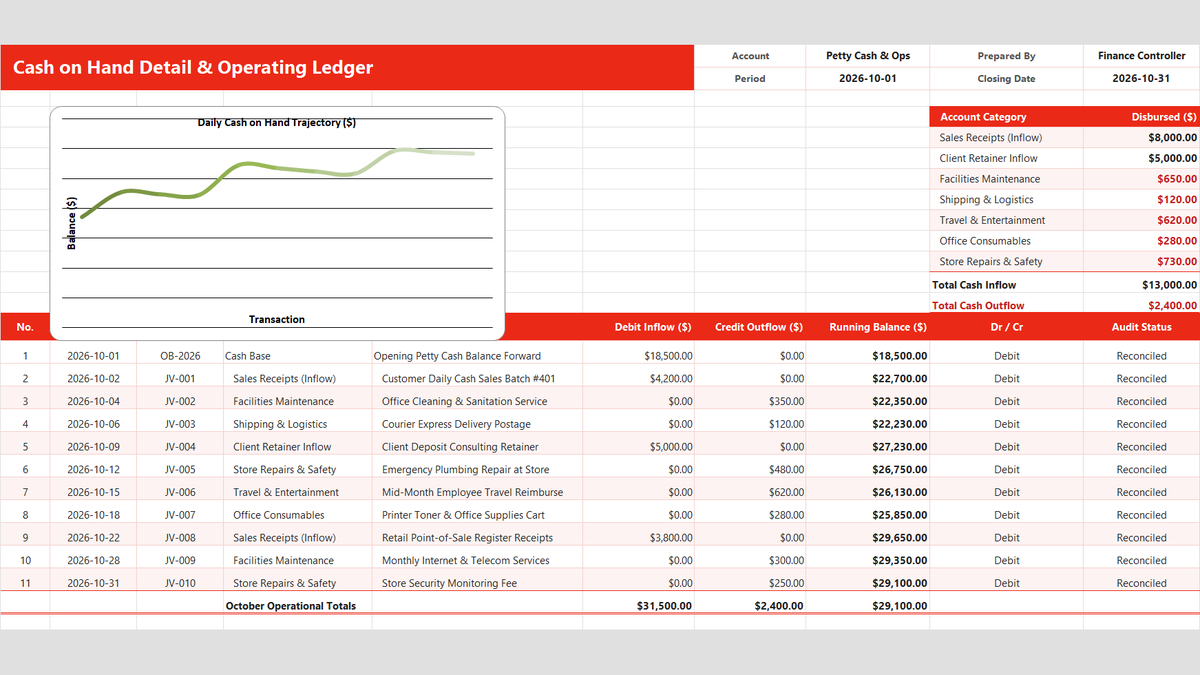
In the top right corner of our sheet (cells J8:K14), we have a clean summary table. We use the versatile =SUMIF() function to add up only the numbers matching each specific category.
In cell K8 (next to Facilities Maintenance), type: =SUMIF($D$17:$D$27, J8, $G$17:$G$27).
Notice the dollar signs ($) locking our ledger ranges. When you copy this formula down to other rows, the category reference (J8) adjusts naturally, while the source data ranges stay firmly anchored. In our example, Excel reports $650.00 for facilities, $120.00 for shipping, and a total monthly outflow of $2,400.00.
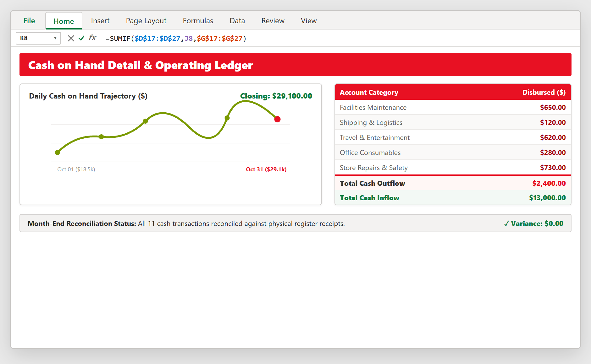
Figure 4: Executive category expense breakdown using =SUMIF() and cash trajectory line chart matching our workbook.
Daily Closing Habits & Petty Cash Best Practices
A good spreadsheet is only as reliable as the daily habits behind it. To keep your cash records clean and stress-free, follow these three simple workplace rules:
1. The Five-Minute Daily Till Count: At the end of every shift, count the physical currency in your cash box before leaving. Your total should match the bottom line of cell H27 ($29,100.00). If there is a small discrepancy, check today paper receipts first.
2. No Cash Out Without a Paper Voucher: Never take cash from the drawer without putting a signed slip or store receipt in its place. Writing the voucher number (like JV-002) in column D creates a clear paper trail that anyone can verify.
3. Lock Prior Months to Avoid Accidental Edits: Once a month is closed and reconciled, use Excel Sheet Protection (Review tab > Protect Sheet) to prevent team members from accidentally modifying historical rows.

Spreadsheet educator and web developer passionate about hands-on interactive spreadsheet practice.
Related Practical Exercises
Explore more hands-on spreadsheet models with downloadable practice workbooks.
 Finance
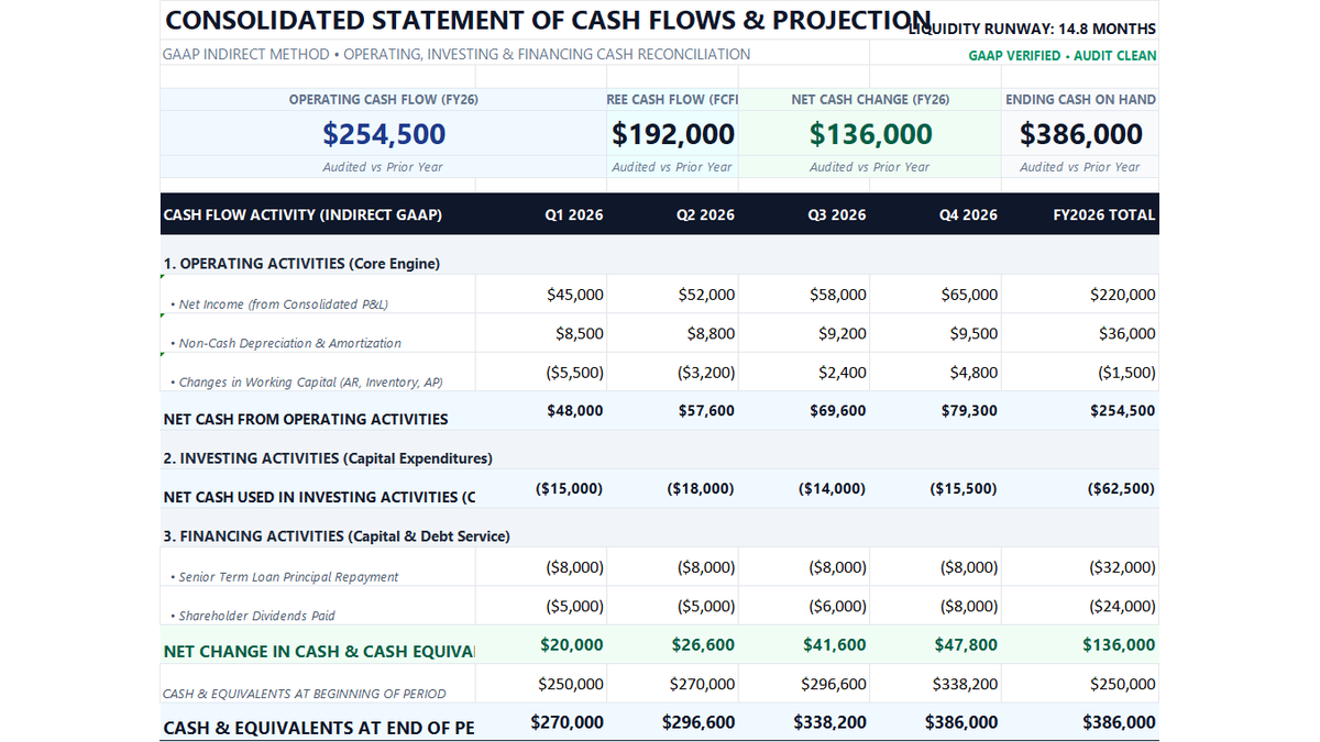
12-Month Cash Flow Statement Excel Template
Learn how to construct a GAAP-compliant 12-month indirect cash flow statement in Microsoft Excel featuring working capital rollforwards, Free Cash Flow to Firm (FCFF), liquidity runway defense, and executive treasury scorecards.
 Finance
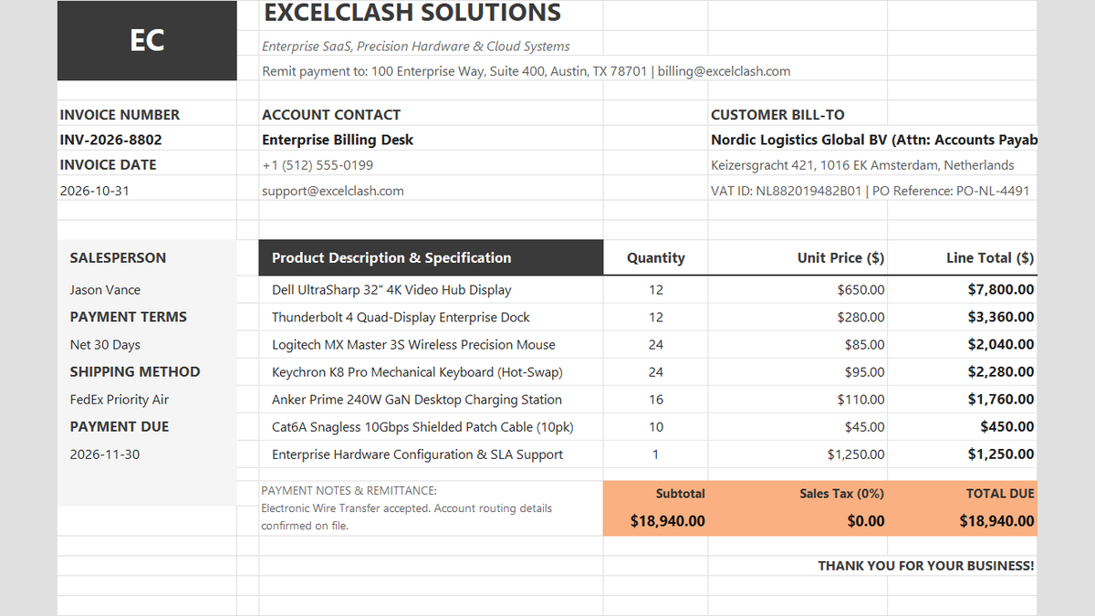
Commercial Sales Invoice Calculator Excel Template
Tired of billing disputes and calculation errors holding up payments? Learn how to build a clean Commercial Sales Invoice in Excel that automatically computes line item subtotals, reconciles sales taxes, and presents payment terms clearly for corporate finance teams.
 Sales
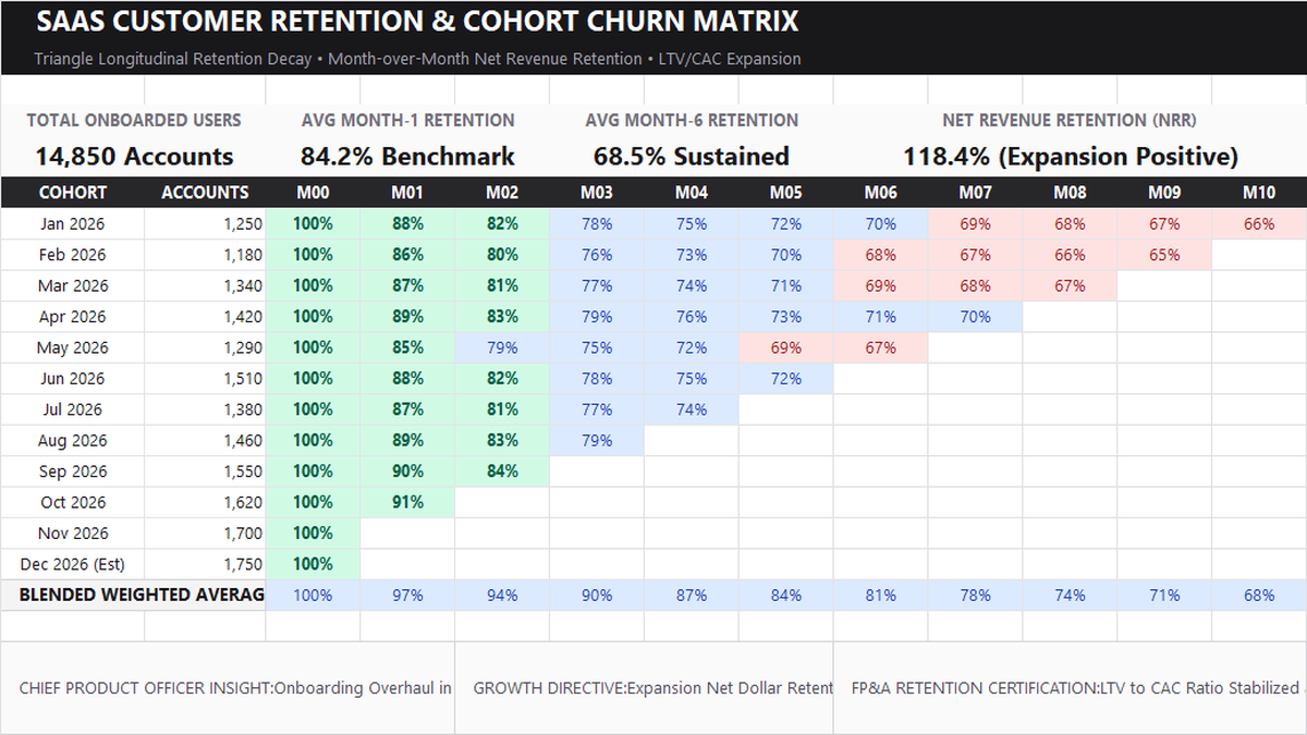
Customer Retention Cohort Analysis Excel Template
Learn SaaS subscription cohort modeling in Microsoft Excel. Build a triangular longitudinal customer retention matrix, calculate Month-1 through Month-10 decay rates, configure multi-color gradient heatmaps, and track executive LTV/CAC expansion metrics.
 Operations
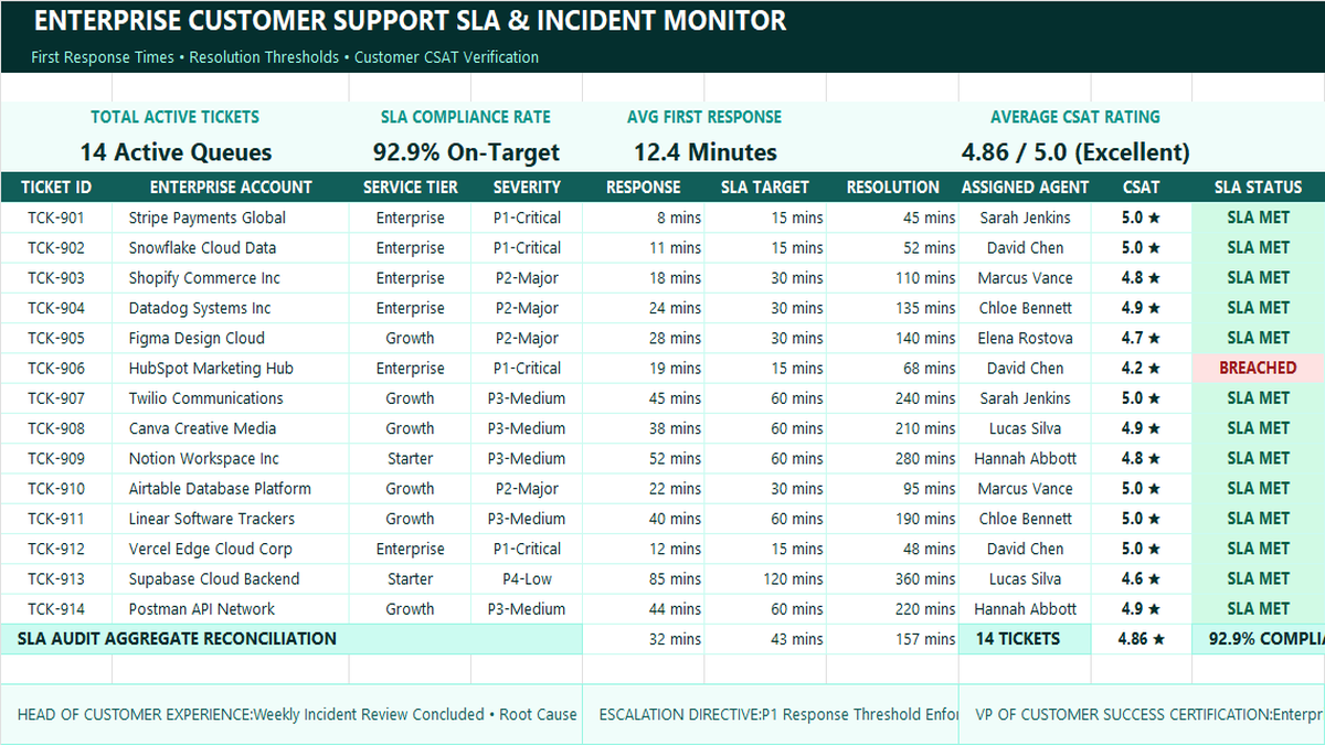
Customer Support SLA Tracker Excel Template
Learn how to build an enterprise customer support SLA tracker in Microsoft Excel featuring severity-based response thresholds, automated breach alerts, team velocity metrics, and CSAT satisfaction scorecards.
 Operations
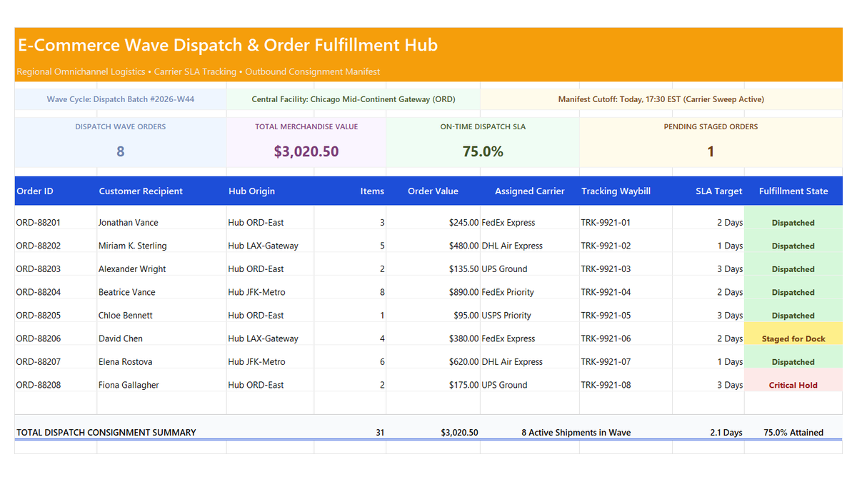
E-Commerce Order Fulfillment Tracker Excel Template
Learn how to engineer an e-commerce order fulfillment tracker in Microsoft Excel featuring wave dispatch cycles, carrier SLA attainment ratios, staged order monitors, and fulfillment manifest scorecards.
Discussion
Ask questions, share formula tips, or discuss alternative approaches with fellow spreadsheet builders.
Loading discussion...